DIF Review and Analysis of Racial Bias in Wordsum Test using IRT and LCA

As reviewed in my previous article, the majority of studies on measurement bias, either on the item- or subtest-level, reached an agreement about the fairness of IQ test. Unfortunately, even among studies which use acceptable Differential Item Functioning (DIF) methods, the procedure was often sub-optimal. This probably leads to more spurious DIFs being detected.

The advantages (and shortcomings) of each DIF method are presented. The GSS data is used to compare the performance of the two best DIF methods, namely IRT and LCA, at detecting bias in the wordsum vocabulary test between whites and blacks.

CONTENT

1. The complexity of DIF detection.

1.1. Item Characteristic Curve.

Traditionally, the probability (P) of correct response at given (latent) ability is expressed as P(θ) for any group for each studied item. DIF is thus expressed as Pfi(θ)≠Pri(θ) for focal (f) and reference (r) group at any given item i, and θ for the latent ability/trait. Sometimes, the formula is given as P(u = 1 | θ) which means the probability of scoring 1 at any given level of the latent score. When the matching criterion is an observed variable, it is given P(u = 1 | X). The focal group is usually the group against which there is bias (having lower score means). The amount of DIF can differ at any given level of θ. Graphically, the two kinds of DIF can be illustrated as follows.

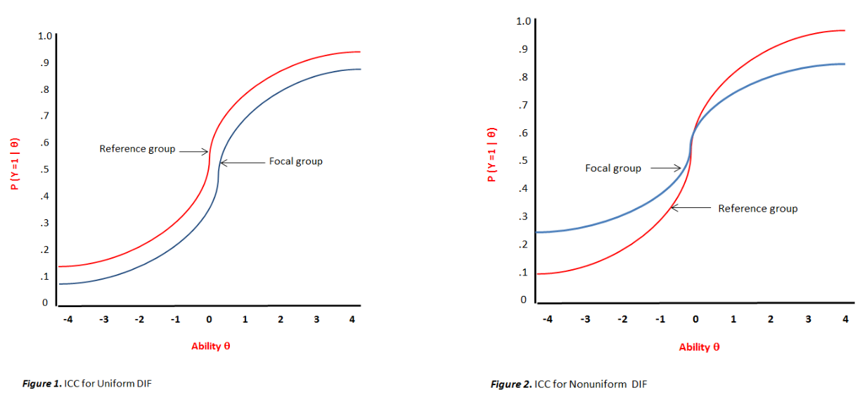
This is a classical IRF (Item Response Function) or more generally named, ICC (Item Characteristic Curve). When the ICCs are summed, it produces a test curve (TCC). The Y (vertical) axis is the probability of correctly answering the item. The X (horizontal) axis is the slope. The left part of the graph shows uniform bias, where the two groups differ on the item’s correct response probability to the same extent at all levels of the total ability score. The right part of the graph shows the situation of non-uniform bias where the magnitude and direction of bias depends on the level of the total ability score. The “areas” between the curves can be taken as a measure of DIF effect size.

Uniform DIF can be simulated by modeling an equal discrimination (a) combined with unequal difficulty (b) parameter across groups. Non-uniform DIF can be simulated by modeling an unequal discrimination (a) combined with equal difficulty (b) parameter across groups (Jodoin & Gierl, 2001, Table 2).

More complex DIFs involve non-unidirectionality. Within non-uniform DIF, there is a point where the two curves have crossed, and before this point the bias favors Group1 but after that point the bias favors Group2. In this case, the DIF is not unidirectional and is termed crossing non-uniform DIF, or non-uniform symmetrical DIF (as opposed to asymmetrical non-uniform DIF in the absence of crossing curves) when ICC areas are cancelled by DIFs going in both directions. In its essence, non-unidirectionality implies non-uniform DIF, because in uniform DIF, the curves cannot cross each other. The location where DIF occurs is important especially when considering DIF cancellation. As Chalmers (2016, p. 21) made it clear, a test is not invalidated if bias occurs at locations with low population density such as the extreme tails.

The uniform DIF has a desirable property that its computation produces unidirectional bias towards one particular group. The crossing DIF is less desirable because the traditional way to compute its total effect is to square the difference which can only produce the unsigned effect size. The signed effect of crossing DIF on the other hand reflects the group difference after accounting for DIF cancellation. Thus, a TCC that is the sum of ICCs, if composed of multiple crossing DIFs, is not easy to interpret.

The modern DIF methods available to statisticians are effective. Despite this, Finch & French (2008) noted that these commonly used methods do not detect well the two types of DIF when both DIFs exist in the data. After simulating the performance of IRT, SIBTEST, LR and MH, they concluded: “It must be noted that the presence of DIF in this context means that the relevant item parameter values differ between the groups (difficulty for uniform and discrimination for nonuniform). Thus, when item difficulty parameters were not different between groups (uniform DIF was not simulated), but item discrimination values did differ, uniform DIF was detected at very high rates. Likewise, when the discrimination parameters were simulated to be equivalent between groups but difficulty was varied, nonuniform DIF was detected at high rates.” (p. 756). At first glance, it only matters if one needs to understand the nature of DIF. As noted above, non-uniform DIF is not desirable and is much less straightforward to interpret.

DIF itself is not problematic if its impact on the composite total score or predictive validity is negligible (Roznowski & Reith, 1999). When a set of items constantly (dis)favors one group, and the combination of these DIFs has an impact on the total score, there is DIF amplification. An outcome deserving investigation. Without noticeable impact, the unavoidable tendency for measures to be related to nontrait variables does not in it self justify the removal of the items.

1.2. The A-B-C-parameters.

In the Item Response Theory framework, the position along the X axis represents the item difficulty (b-parameter) or the amount of the total score needed to get the item correct. The slope is the item discrimination (a-parameter) among levels of total score. The steeper the curve and the more discriminating the item is between the groups. The Y intercept (the location where the slope crosses the Y axis) or c-parameter is the guessing parameter (sometimes called the lower asymptote), the probability of correct answer for low-ability persons. It is assumed that the probability of correct response will diminish when the item difficulty increases for low-ability subjects compared to high-ability subjects. In general, simulation studies put the c-parameter at 0.20.

Stated otherwise, uniform DIF is observed when the group effect (equivalent to the b-parameter) has a nonzero coefficient on the dependent variable (the item), holding constant the test total score. Non-uniform DIF is observed when the interaction between group effect and total score (equivalent to the a-parameter) is non-zero, holding total score constant. Non-uniform DIF occurs rarely in practice (Hidalgo & López-Pina, 2004) but its consequence shouldn’t be ignored. All types of DIF must be investigated.

In bias study, one should guard against misleading interpretation of group difference in parameter(s) as indication of bias. According to Linn et al. (1981, p. 171), what matters is the difference in the item’s correct response probability and this is not always related to differences in the abc parameters. In their words: “It is possible, as was sometimes observed in the present study, for item parameters to be substantially different yet for there to be no practical difference in the ICCs. This can occur, for example, where the b parameter is estimated to be exceptionally high for one group. To illustrate this, consider the following pairs of hypothetical item parameters for two groups in terms of a common θ scale: group 1, a = 1.8, b = 3.5, and c = .2; group 2, a = .5, b = 5.0, and c = .2. The item difficulties and discriminations for the two groups are markedly different; but the difference in the ICCs is never greater than .05 for θ values between -3 and +3.” The likely reason for this outcome is that the item difficulty was too high and therefore inappropriate as opposed to an item that would match the examinee ability (Hambleton et al., 1991, p. 112).

In the literature, we usually encounter technical wordings, such as “the response data follow Rasch (1PL) model”. All this illustrates is that the item response is explained solely by the difficulty parameter. Rasch or IRT generally assumes strict unidimensionality. The IRFs in the above picture, for example, don’t follow a Rasch model because discriminations are not similar.

When a test is subject to potential guessing, it has to be modeled. Not all DIF methods can account for guessing. DeMars (2010) illustrates the problem with this graph:

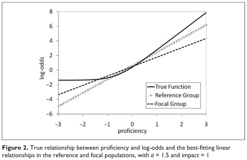
The solid line represents the true log-odds for a 3PL item. The two other lines the best fitting lines for reference and focal group under 2PL model. DeMars displays this graph to illustrate what happens if a model such as 2PL fits the best linear relationship. In this case the slope will be underestimated (especially for the group for whom the item is more difficult) to accommodate the data points influenced by the nonzero lower asymptote. This bias is stronger as impact is greater.

It has been argued somewhere that the 3PL is useless because it fails to distinguish between random and informed guessing. However, random guessing happens when low(er) ability persons do not know the answer to an item that is beyond their capacity whereas informed guessing happens when high(er) abiliy persons have partial knowledge or synthesize information from other sources such as prior information in the item (e.g., wording cues or distractors). Jiao (2022) reviewed studies showing that adding a fixed lower asymptote to the Rasch model increases the accuracy of ability parameter estimation. Using simulations, Jiao demonstrated that the extended Rasch model in which a constant guessing parameter is introduced can well recover the true model parameters. This finding is important because Rasch has desirable properties, such as consistency, that other IRT models do not possess.

For any given level of total score, if the reference group has a higher % correct than the focal group in some items, the focal group must have a higher % correct on other items. Otherwise, the examinees would not have the same total score level.

1.3. Matching for total score with measurement error and bias.

Many studies on test bias failed to properly equate the groups, resulting in more DIFs being detected, with the wrong pattern of probabilities, and perhaps even the wrong items being detected. Not accounting for measurement error, not excluding DIFs, not controlling for multiple dimensions are the typical causes of improper matching.

Two ways exist to equate the groups in total score, either using observed (manifest variable) score or a latent (variable) score. The difference between the two approaches seems to increase with decreasing reliability, causing type I errors. DeMars (2010, Figure 1) informs us that the less reliable the test is, and the less % of variance of the latent score would be explained by the observed score. DIF methods based on manifest variables are not recommended unless the test has very high reliability.

Whether we should include the studied item in the total score matching is a good question. DeMars (2010) explains: “Including the studied item in the matching score makes a difference because conditioning on Item i plus 20 other items is not the same as conditioning on 20 other items that do not include Item i. There is a statistical dependence between the total score and the item score, which must be taken into account. This is most obvious when thinking about a score of 0. If Item i is not part of the matching score, some proportion of those in the 0 group could get Item i right. But if Item i is part of the matching score, none of the examinees in the 0 group could have answered Item i correctly.” (p. 965). The inclusion of the studied item seems theoretically preferable.

Generally speaking, the high occurrence of type I error misleads DIF analyses. That was mainly due to significance tests. When they were combined with an effect size, false positives (FPs) decrease. Another way to deal with type I errors is to use a 2-step purification procedure. First, use the total score to screen for potential DIFs. Second, re-compute a new (purified) total score with only the DIF-free items for the final analysis. The items used (DIF-free) to build the purified total score matching are called “anchor” items. If the matched total score includes DIFs during the first step of DIF screening, the variable is internal, as opposed to external if it contains no DIF. Shih & Wang (2009) noted in this regard, “In practice, a matching variable is often (if not always) internal because it is very difficult to find an external set of DIF-free items that measure the same latent trait for which the studied test was designed”. They still conclude that purification is effective. One problem is that the general procedure to perform this purification relies on significance test instead of examining relative model fit indices or effect size categorizations. Both Finch (2005) and Shih et al. (2014) found evidence of increased type I errors when the matching (or anchor) test variable contains more DIFs. They suggest to retain in the matching variable the items having the least “deviance” or χ² difference.

When the test is multidimensional, more than one ability is measured. The overall total score can be measuring a large portion of the variance in each subtest scores but a minor variance of some would be best explain by a particular dimension (e.g., represented by a certain (set of) subtest(s) within the test) not entirely explained by the total score. In this case, more items are falsely identified as DIF when total score is used as matching variable than when an individual subtest is used, which application is even less optimal than using multiple subtests simultaneously as criterion matching. This is what Clauser et al. (1996a) concluded with regard to LR method in their study of the items on 4 content-specific subtests of medical competence. Additionally possible is the inclusion of some background or SES variable, for example, in the logistic regression (Clauser et al., 1996b, p. 456). If DIF disappeared when education is added in LR equation, it means that some known or unknown factors closely related to years of education fully explain the DIF.

Local dependence between items, which violates unidimensionality, is also a potential bias yet rarely discussed. It occurs when several items form one (or more) cluster(s) within a test or even subtest, called bundle(s) or testlet(s), causing the response of these items to be dependent on one another. If conditional on ability the testlet score differs across groups, one must investigate whether the test was measuring two (construct-relevant) abilities and if not the test truly exhibits bias. The multilevel approach can model items at level 1 and individuals at level 2, eventually adding schools at level 3 while modeling dependencies using dummy-coded testlet variables (Beretvas & Walker, 2012). Another method is to simply add a random effect to the logit equation of IRT that is an interaction of person with testlet (Wainer & Wang, 2001).

2. Statistical procedures.

2.1. ANalysis Of VAriance (ANOVA).

An earlier technique was the ANOVA. Like LR, the item must be the dependent var., the total score and grouping variables as independent variables. Usually, in ANOVA framework, the dependent is a continuous variable (e.g., test score) and the independent variables are dichotomous or categorical, such as groups and items. Eta-squared values (i.e., variance accounted for) larger than 0.02 would be evidence of small bias, and larger than 0.06 for moderate bias, if this large Eta-square is associated with the group*item interaction. This would mean that the item have different relative difficulties within each group. There exists two types of interaction : ordinal and disordinal. The first happens when the interaction does not distort the rank order of p-values between groups whereas the second happens when the interaction changes the p-values’ rank-ordering between groups. This method has been cited and used regularly by Jensen (1980, e.g., pp. 432-438, ) in the study of test bias. However, a study of simulated bias conducted by Camilli & Shepard (1987, Table 1) shows that ANOVA’s group*item interaction term is clearly insensitive to biases that add or substract from the true group differences (δ²G). Biases that add to mean group differences can go from zero to some extreme levels, by varying the group differences in item difficulty (i.e., passing rates) and/or number of biased items, and yet ANOVA will consider them as minor changes in the group*item interaction term (σ²G*item) and instead will attribute these biases to the group variance (σ²G). Put it otherwise, ANOVA falsely interprets this biased group differences as real group differences. Another problem is that the probability of bias detection was a function of the magnitude of item difficulty relative to group mean differences. In their example, ANOVA detecting the smallest group*item interaction for the easiest and hardest items whereas such interaction was maximized when the item was of average difficulty, even though the ICC curves were identical for the two groups in all of these items (i.e., no bias). Group difference in difficulty in regions other than between the means can miss the presence of biases. ANOVA can create artifactual biases as it can obscure those biases.

2.2. Transformed Item Difficulty, or Item Correlation Method.

The TID, or Angoff’s (1972, 1982) Delta Plot technique, also regularly used by Jensen (1980, pp. 439-441, 576-578) consists in correlating the rank-ordering of item difficulty or passing rates (sometimes ambiguously termed “p-values” or simply “p”) between the two groups studied. Having the p-values and using tables of the standardized normal distribution, the normal deviate z is obtained corresponding to the (1-p)th percentile of the distribution, i.e., z is the tabled value having proportion (1-p) of the normal distribution below it. Then to eliminate negative z-values, a delta value is calculated from the z-value by the equation A = 4z + 13. A large delta value indicates a difficult item. If all items on a test have a similar relative difficulty for the two groups, the plot exhibits a 45° trend-line. Deviations from this line (i.e., outliers) would indicate bias. A correlation close to 1.00 would suggest that the relative item difficulty in one group does not differ from another group; what is easiest/hardest for one group is also among the easiest/hardest items for another group. Hence the conclusion that the test behaves the same way in both groups. One problem with the method is that the “p” differences tend be magnified when item discrimination increases, so that artifactual bias may appear just because the item becomes more discriminating. Even when the items were initially unbiased, the discrimination parameter can make them biased. This technique would be more valid when conducted for two groups that do not differ in mean ability or if all items are equal in discrimination (a-parameter constant across groups). After establishing the inferiority of TID compared to IRT, Shepard et al. (1985) explain in these words : “Although the delta-plot procedure seems to match perfectly with the relative-difficulty conceptualization of bias, it has been shown to be a poor index because it will produce spurious evidence of bias (Angoff, 1982; Hunter, 1975; Lord, 1977). The misperception of bias occurs because the p-values are as much a measure of group performance as they are a characteristic of the test item. If groups differ in mean ability, then items that are highly discriminating will appear to be biased because they better distinguish the performance of the two groups.” (p. 79). High discrimination can cause type I error whereas low discrimination can cause type 2 error (real DIF not detected by TID).

Because of the troubles caused by item discrimination, Angoff (1982) proposed a possible improvement of TID by dividing the transformed p-value by the item-test correlation. Seemingly, the procedure is aimed to correct for the false positives generated by variations in item discrimination. Shepard et al. (1985) noted this method did not improve agreement in bias detection with other methods, such as ICC. They recommend another method; regress out the (combined-group) item-test correlation from the Angoff TID p-values. The residual delta indices are then calculated as the difference between the observed index and the expected delta value based on the item’s point biserial. And yet, this modification was still inferior than the (signed) χ² method in bias detection agreement.

Ironson & Subkoviak (1979, Figure 1) compared what kind of items will be detected as biased by ICC method and Angoff’s Delta Plot method. The difference is striking. There must be no doubt this method should never be used. Nonetheless, Magis & Facon (2011) attempted to improve the Angoff’s Delta Plot. First, they begin to describe its peculiarities, and noted that if the groups differ in item discrimination, non-uniform DIFs will probably not be detected. In extreme cases, where all subjects either get the item 100% right or 100% wrong, the delta scores become infinite.

Obviously, this shortcoming was not a fatal flaw to TID because artificial biases are simply created (Type I error) not eliminated, and Jensen (1980; & McGurk, 1987) as well as Rushton (2004) found little or no evidence of bias (in either direction) using this method. But more damageable is the fact that TID can detect biases in the wrong direction, e.g., against the majority group instead of the minority group. Another serious drawback is that non-uniform DIF will not be detected.

2.3. Partial Correlation Index.

Stricker (1982) was an advocate of the technique. This simple test consists in correlating the group variable (e.g., coded 0;1 or 1;2) with the item, when controlling for total score. One of its strength is its flexibility (any number of different kinds of subgroups can be accommodated simultaneously; and the subgroups can be represented by dummy-coded categories, e.g., race, or quantitative variables, e.g., socioeconomic status) and its simplicity in both computation and interpretation. However crude this method looks, the index correlates, agrees strongly with the ICC index in detecting DIFs. Stricker uses a test of significance for Phi coefficient (with 1 df) in the detection of DIF; Jensen (1980, pp. 431-432, 459-460) gives the calculation of the Phi and its significance test. The partial correlation provides a direct estimation of the effect size. If the group-item correlation is large, we might expect a group effect, and DIF would be suspected. Nonetheless, it remains unclear how this technique could detect non-uniform DIF. Stricker (1982, p. 263) recognizes it. However, dividing the total sample in subgroup ability levels can partially solve this problem.

2.4. Chi-Square (χ²).

Shepard et al. (1985) describe the Scheuneman’s procedure in these words: “The chi-square bias method is a rough approximation to the IRT method. It follows the same definition of unbiasedness; that is, individuals with equal ability should have the same probability of success on a test question. Rather than a continuous ability dimension, however, the total score scale is divided into crude intervals, usually five. Within these intervals, examinees from different groups but with roughly equivalent total scores are expected to have equal probabilities of success on the item. An expected set of proportions is calculated for the two-fold table in each interval (ethnic group by correct/incorrect response) assuming independence. Then the conventional chi-square is calculated based on the 2×2 table within each ability interval and finally these chi-squares are summed across ability levels. Large deviations from expected frequencies within ability strata will lead to large bias indices. A signed chi-square statistic was also obtained by signing the direction of bias in each interval and then summing the chi-squares across intervals. As with other signed indices, if the direction of bias is not consistent across intervals opposite biases in different total-score regions will cancel to some degree. … The significance of the chi-square values would be even more difficult to interpret for signed indices where the canceling of positive and negative values has no counterpart in statistical distribution theory.” (pp. 81-82).

Shepard et al. (1985) attempted to improve this method by using the first unrotated component score derived from PCA, instead of the observed total score. But that did not improve Chi-Square and made things worse. They also attempt to increase the number of (total score) intervals by 10 instead of 5. Again, no improvement was apparent. They finally use another strategy to improve it. The DIFs detected with χ² are removed from the total score, and this new observed (unbiased, purified) total score is used to match the groups. The improvement in its agreement (correlation) with IRT in DIF detection is not compelling.

2.5. Expert Judgment.

Conoley (2003) explains the method in these terms: “The method of using expert judges involved selecting individuals who represented a gender group and/or a different ethnic minority group or had special expertise about a particular group. These individuals were asked to rate items on their offensiveness or likelihood of being biased against a particular group (Tittle, 1982).” (p. 26). Conoley assembled a panel of 10 teachers (mean years of experience = 17) as judges (5 experts, 5 non-experts) for deciding which items could be biased against the ELL mexicans as compared to whites. To compare the accuracy of their judgement from what the partial correlation indices actually reveal, the unweighted kappa coefficients were used. None of the judges could adequately predict the items that would be biased against ELL mexicans based on the partial correlation method of DIF. Whether the lack of agreement between judgments and statistical results can be (partially) due to suboptimal statistical procedures is difficult to tell. While this method is now viewed with skepticism, it is sometimes suggested as a DIF method prior to purification.

2.6. Standardization P-DIF method.

The technique, DSTD or STD P-DIF, is similar to MH and has been proposed by Dorans et al. (1986, 1992) and consists in computing the passing rate (p) difference between groups controlling for total score for groups with equal total score. The following formula is applied : DIF_STD=∑[ωfs*(Pfs-Prs)]/∑ωfs where Pfs-Prs is the (proportion) relative frequency of correct response calculated as the number of subjects at score group level “s” (also denoted x or k) in focal/reference group who scored 1 (i.e., the absolute frequency of correct response) on the item divided by the total number of subjects in the focal/reference group, and ω is the weighting factor at score group level s supplied by the standardization group to weight differences in performance between focal and reference group. Several weights can be used : 1) the number of examinees at s level in reference group 2) the number of examinees at s level in focal group 3) number of examinees at s level in the total (focal+reference) group. Dorans recommends 2) because it provides the greatest weight to differences at those score levels most frequently observed in the focal group. Spray (1989) also used this weight and found that the P-DIF along with MH statistics are viable indicators of DIF. The formula expresses the standardized p-difference between the groups and yields an index ranging between -1;+1. Positive values indicate the items favor the focal group, and negative values indicate the items favor the reference group. Values between -0.05;+0.05 are negligible, values between -0.10;-0.05 and +0.05;+0.10 are moderate, and values outside the range -0.10;+0.10 are serious. As in the case with MH, the STD P-DIF requires the construction of different categories in the matching (total score) variable, such as 5 levels (denoted “s”) of ability, i.e., 0-2, 3-4, 5-6, 7-8, 9-10, in order to get the best matched grouping as possible. The STD P-DIF should not be confused with IMPACT, expressed as IMPACT=∑(ωfs*Pfs)/∑ωfs-∑(ωrs*Prs)/∑ωrs, and which is the between-group difference in total item difficulty. However appealing the P-DIF appears, the SIBTEST was an improvement of this technique.

2.7. Logistic Regression (LR).

A popular technique for DIF detection is the logistic regression (LR). The model would be expressed as [EXPodds/(1-EXPodds)] ln[P/(1-P)] = β0+β1(θ)+β2(g)+β3(θg), where β0 is the constant, β1(θ) total score, β2(g) group variable, β3(θg) interaction between group and total score (i.e., the product of the two variables) and where EXPodds is the exponential of the odds. The item is the dependent variable, i.e., the outcome to be predicted. In model 1 (said, the compact model), only the predictor β1 is considered, in model 2, we add β2, in model 3 (said, the augmented model), we add β3. The absence of DIF would be indicated by parameters β2 and β3 equal to 0 in model 3.

The situation becomes more complicated when the test measures more than one ability. In such a case, Mazor et al. (1995) and Clauser et al. (1996a) recommend for LR the inclusion of a second ability (sub)test score. These authors discovered that such procedure helps to remove the detection of spurious DIFs created by only including the total test or a single subtest score. In the LR framework, the formula including interaction terms may be expressed as: β0+β1(θ1)+β2(θ2)+β3(g)+β4(θ1g)+β5(θ2g). That is, the subtests (θ1, θ2, …) must be entered at once. Clauser et al. (1996a) found this matching strategy to be the most accurate. Subtests ideally must have enough reliability. However, the multidimensional LR displays too large type I error and low power in detecting non-uniform DIF even for 2PL data (Bulut & Suh, 2017).

The common statistics reported for the assessment of DIF is the p-value associated with the 1-df χ² difference between models, say, 2 vs 1, or 3 vs 2, whereas the 2-df χ² test is not the most recommended because it compares directly model 3 with model 1. On this matter, Jodoin & Gierl (2001) write: “Swaminathan and Rogers (1990) noted that “In the LR model, the interaction term may adversely affect the power of the procedure when only uniform DIF is present because one degree of freedom is lost unnecessarily” (p. 366). Working under the premise that an effective effect size measure can control Type I error, it seems reasonable to modify the 2-df chi-square test into separate 1-df tests of uniform and nonuniform DIF, respectively. Theoretically, this change should result in superior power in the detection of uniform DIF with little change in the Type I error rate if an appropriate effect size measure is found.” (p. 332). They also explain that group and total score must be centered or standardized, in order to avoid collinearity with the interaction term, which in this case uses the interaction with the two z-score variables. Both Jodoin & Gierl (2001) and Gómez-Benito et al. (2009) showed that the traditional use of likelihood ratio increment (i.e., -2*log(likelihood ratio) or Logistic Regression Chi-Square between model 1 (total_score) and model 3 (total_score + race + race*total_score) results in an overestimation of false positive (i.e., inferring bias when there wasn’t any) and that, instead, regarding the R² increment between models reduces the false positives. Specifically, this χ² difference is given by the difference in -2Log Likelihood (-2LL), sometimes called “deviance”, in the models (full vs reduced) being compared. Zumbo (2008) remarked that the common criterion for researchers today is: to be classified DIF, regardless of the kind of DIF, the 2-model (i.e., model 3 minus model 1) χ² difference must have p-value ≤0.01. This online calculator can give us our p-value, by just entering the χ² (here, -2LL) difference and the df (difference in number of variables between the models). Unfortunately, larger sample size results in larger χ² values and by this, larger model χ² differences as well. A significant DIF is of no concern if the magnitude of DIF is not large.

But the most important output is the increment (Δ) R² between the models. If race (or its interaction with ability) is a meaningful predictor of the item response, independent of ability, the R² should increase by a large enough amount. LR does not provide the traditional R² but instead a pseudo R², e.g., the Nagelkerke R². This value expresses the unexplained % of variance that has been decreased by the set of (independent) variables, so the larger the better. Meaningful predictors must cause the Nagelkerke to increase. The Cox & Snell R² gives the same information but its upper bound value is less than 1.0, and is therefore less recommended. Zumbo and Thomas (1997) propose an assessment criterion with three categories: negligible DIF if ΔR²<0.130, moderate DIF if 0.130≤ΔR²≤0.260 and large DIF if ΔR²>0.260. And the three categories proposed by Jodoin and Gierl (2001): negligible DIF if ΔR²<0.035, moderate DIF if 0.035≤ΔR²≤0.070 and large DIF if ΔR²>0.070. These estimates are based on the correlation between the LR R² and SIB effect size.

Unfortunately, even with this criteria, Hidalgo & López-Pina (2004, Table 4) demonstrate that the ΔR² in LR has more tendency to flag DIFs as small DIFs than the MH effect size which has more tendency to flag these same items as moderate and large DIFs. None of the above suggested cut-off values provide satisfaction. Perhaps the problem is the R² itself. Gómez-Benito et al. (2009, Table 2) show that LR effect sizes result in 0% of correct identification (CI) of DIFs with Zumbo & Thomas criteria whereas Jodoin & Gierl also produce disappointed results, for every types of DIFs. Generally, when N increases, the proportion of CI decreases, even tending towards zero. That is, LR performs best when N is small when relying on R². The CI can be even lower than tests of significance. The CI increases when N increases if we rely on significance test. The CI rates also increase when DIF size increases. But even under the condition of low-to-moderate DIFs (0.1 to 0.4) the CI for R² was not higher than 2% or 10%, depending on types of DIF whereas the significance test has a CI between 13% and 60%. The proposed cut-off must be too generous if R² behaves so badly. Therefore, I propose the following cut-off values: negligible if ΔR²<0.005, moderate if 0.005≤ΔR²≤0.010 and large if ΔR²>0.010. These approximative values are based on the cut-off comparison between LR and IRT in Oliveri et al. (2012; Table 2).

Due to the shortcoming of R², Hidalgo et al. (2014) decided to follow Monahan et al. (2007) recommendation for a new effect size, the delta log odds ratio, which is inspired by MH effect size (odds and delta). The odds ratio is calculated as follows in LR: άLR=EXP(β2). β2, remember, is the coefficient for the group variable. And the delta as follows: ΔLR=-2.35*LN(άLR). Hidalgo et al. (2014) recommend it because this effect size, compared to the usual R², results in a much higher power and correct identification of DIF, even if the log odds ratio shows higher FPs than R² when N is extremely small (e.g., 100/100 or 250/100) or Ns were both small and very unequal (e.g., 500/100) but no such inflated FPs were apparent when N are 250/250 or 500/250 or 500/500. The FPs for R² are always kept at (near) zero under all conditions except N=100/100. The cut-off guidelines for these new indices are the same as for Mantel-Haenszel. The index, however, is only applicable to uniform DIF. The index and formula for the LR odds ratio in non-uniform DIF have not been studied yet.

Likewise, DIF and DTF plots are more useful than ΔR² at identifying DIF. Oliveri et al. (2012, Table 2) compare the effect size measures used in parametric IRT, non-parametric IRT and ordinal LR. When IRT effect size detects a moderate or even a large DIF, LR will see it as very negligible given the actual cut-offs. The best example is the ICC presented in Oliveri’s Figure 3. A simple look at the graphs shows how large the ICC gap is and yet the LR ΔR² was only 0.018 when the P-diff in IRT was -0.119 with cut-off P-diff≥0.100 (absolute) for large DIF. Either that means R² should never be used or that appropriate cut-offs must be defined. That is why I recommend a very stringent cut-off with ΔR²>0.010 for large DIF. At the same time, however, DIF and DTF plots derived from the two IRT and LR produce similar results in identifying the pattern of DIF.

The same authors (see also; Zumbo, 2008) show and explain how to create some IRT/LR graphical DIF and DTF. We must “save” the predicted category score from the model 3. We then create a scatterplot with the predicted item response on Y-axis and total score (or alternatively, the item-corrected total score) on X-axis. Finally, we use the grouping variable as marker variable in order to create separate plots for each groups. A further step can be processed to create the graphical LR DTF by computing the total predicted test score which is simply the sum of all of the predicted item responses. Then we create scatterplot with total predicted test score on Y-axis and the observed total score on X-axis, with group variable set as marker. This graph allows us to get a graphical look at the overall impact of all DIFs at the test level.

There is possibility to proceed with an iterative purification in order to control for type I errors. French & Maller (2007, Tables 3-8) showed with respect to LR that purification increases (modestly) power rates for uniform DIF but also decreases (slightly) power rates for non-uniform DIF under various conditions (equal/unequal N, equal/unequal group means, % and magnitude of DIFs). Power, of course, increased with N. They also discover (Table 2) that false positives (FPs) decrease very slightly with the combination of significance test and purification compared with the situation where significance test only is used, under the condition of equal ability between groups. However, when the groups initially differed in total score, the purification does not reduce FPs or improve power rates under virtually all conditions. They discovered that the type I error rates, usually thought to be high in LR, equal zero with a combination of significance test and effect size, and this type I error holds in various conditions, whether N increases, or DIF at 10% or 20%, with DIF magnitude varying from modest to large, i.e., 0.40, 0.60, or 0.80, and whether or not the two groups differ in total ability/score distribution. There is no large FPs increase for significance tests with N when the two groups have equal ability, but large FPs increase for significance tests when N increases. Gómez-Benito et al. (2009, Table 2) reported FPs close to zero for R² except when N is 100/100 whereas significance test yields FPs of slightly higher values than 0.05 even though it does not increase with N, under all conditions.

One other reason of FPs with R² is the non-use of latent score in the traditional LR method. DeMars (2009, Table 2) proposed the SIBTEST correction for LR, which consists in correcting the total score and the item response from measurement errors. DeMars analyzed the outcome on effect size (Δ) and its average standard error (in SD). When there was no group impact, the average estimate of Δ was unbiased for all DIF methods regardless of corrections. But under group impact condition, the linear correction reduced the bias in Δ estimates, and the nonlinear correction reduces it even further. The linear correction reduced the bias in SD and the nonlinear correction performed better only when both sample size and impact were large. The nonlinear correction increased bias in SD with small sample (N=250) or when impact was absent. The regression correction did little to improve the Type I error rate for detecting nonuniform DIF using LR. The lack of a guessing parameter in the LR model would seem to contribute to this problem. This is why data with guessing cause inflated FPs in LR (DeMars, 2010).

To account for guessing, Drabinová & Martinková (2017) proposed the non-linear regression (NLR) as a proxy of 3PL IRT model. This procedure calculates the probability of guessing right without necessary knowledge, allowing lower asymptote to differ from zero. Their newly developed difNLR (for R) was evaluated against LR, MH, and two IRT methods such as Lord’s χ² and Raju’s ICC area in a 3PL simulated data (Table 3). In terms of power, all methods perform comparatively well with N=2000 and more (except MH having no power in detecting non-uniform DIF). As for type I errors, all methods perform well except the two IRT methods at N=1000 and all methods perform badly when N=5000 with several uniform DIFs.

Shih et al. (2014) proposed the so-called DFTD method (“DIF-free-then-DIF”). First, we conduct LR to detect DIF through significance of the χ². Remove DIF items from the new matching variable. Reconduct LR with this new matching variable to study all DIF items individually. Record the difference in “deviance” and select a set of items (depending on the length of the test) with the smallest “deviance” (i.e., difference in models’ -2LL) and add them to the matching variable score to be formed. Those selected items are called “anchored” items. Their simulation evaluates FPs and power for LR standard, LR with scale purification (LR-SP), LR with SIBTEST nonlinear correction (LR-SIB), LR with DFTD (LR-DFTD), LR with DFTD and linear correction (LR-L-DFTD), LR with DFTD and nonlinear correction (LR-N-DFTD).

Under condition of 3PL and impact=0SD, the numbers are virtually identical for FPs except that LR and LR-SIB have lower FPs than under 2PL when %DIF is high (e.g., 30% or 40 %). For power, the numbers are smaller for all methods, and DFTD methods again outperform the others only when both N and %DIF are the highest but very marginally. For power only, LR-SP outperforms DFTD methods in all conditions.

Under condition of 3PL and impact=1SD, the FPs seem larger for all methods, especially when %DIF is high. In the 20-item test, DFTD methods again show worse performance except for LR-L-DFTD which has the lowest FPs among all methods when %DIF is high. But LR-L-DFTD and LR-N-DFTD are still better than other methods in 60-item test. Concerning power (again, compared to 2PL) the numbers are higher in small Ns but lower in high Ns. It is not clear that , LR-DFTD and LR-L-DFTD are better than LR-SP in 20-item test but LR-N-DFTD clearly was the best. LR and LR-SIB perform the worse and LR-SIB is comparably worse than LR in 20 item-test. In 60-item test condition, LR-DFTD and LR-SP perform comparably well and seem to be the best, followed by LR and LR-SIB, whereas LR-L-DFTD and LR-N-DFTD are at the bottom.

The same authors also tested the impact of anchor length (4, 6, 8, 12 items) on FPs and power. Under 2PL and 3PL, when impact=0SD, anchor length only improves power for both LR-L-DFTD and LR-N-DFTD. Under 2PL and 3PL, when impact=1SD, anchor length reduces FPs and power for both LR-L-DFTD and LR-N-DFTD. However, when impact is 1SD, all changes in FPs and power occured when anchor length increased from 4 to 6, and there is virtually no change after this.

So, the general picture was that FPs increase with larger N and smaller test length whereas power increases with larger N and larger test length. Curiously, LR-SIB is no better than LR. The fact that FPs tend to decline with test length (only when impact exists) can probably be attributed to the higher reliability associated with test length. The DFTD seems recommended when test length is large. Keep in mind that power increase is not always beneficial, especially if it is associated with higher FPs.

In simulated 2PL data, Li et al. (2012, Tables 2-4 & Figure 5) examined FPs for LR and MH by varying the discrimination (a) values of both the studied items and non-studied items. When non-studied items have a-values between 0.2 and 1.8, both methods show much larger FPs than when the non-studied items have a-values between 1.2 and 2.0. In both conditions, FPs for both methods increased when the studied item has very low or high a-values. The authors noted that both methods show inflated FPs with samples and impact, and their simulations all assumed N=1000/1000 for reference/focal group and impact of 1SD. They recommend checking for discrimination values prior to conducting DIF.

The Multilevel LR is highly recommended to account for the cluster (i.e., multilevel) structure of the data. When examining between-cluster variables, French & Finch (2010) found that this procedure kept FPs below the nominal rate of 0.05, while LR exhibited extremely high FPs, but at the cost of drastically reducing power rates, compared to using LR, irrespective of DIF size and cluster number or size. However, larger cluster size and number of clusters appear to increase power substantially for both method.

2.8. Mantel-Haenszel (MH).

Another widely used method is the Mantel-Haenszel (MH) procedure. Concretely, MH is based on the analysis of contingency tables, compares item performance of two groups initially matched on total score. In the MH framework, an item shows uniform DIF if the odds ratio (OR) of correctly answering the item at a given score level J is different for the two groups at some level J of the matching variable. The formula of common odds ratio, an index of DIF effect size, is ά=∑(A*D/N)/∑(B*C/N) where N is the grand total sample size, A and B being respectively score 1 and 0 in the majority group, C and D being respectively score 1 and 0 in the minority group (Raju et al., 1989; Nandakumar et al., 1993). The utility of ∑ (“sum of”) reveals itself when we want to pool the odds ratio. For instance, the aggregated ά equal to 1.00 would suggest either the total absence of DIFs or the cancellation of DIFs. The (common) odds ratio ά>1.00 indicates bias against the focal group while ά<1.00 disfavors the reference group.

But MH is thought to be not well suited for non-uniform DIF detection, especially when items were of medium difficulty even though it can detect some few non-uniform DIFs when items were easy or difficult. Initially, MH was designed to detect only the uniform DIF and in this respect has equal power with LR (Rogers & Swaminathan, 1993). While MH is not good at detecting non-uniform DIF, Hidalgo & López-Pina (2004, Table 4) compared the standard MH with a modified MH against LR. The modified MH is aimed to improve MH procedure to detect non-uniform DIF by splitting the sample in two (or more) parts, low-scoring group, high-scoring group, e.g., by taking the mean. Their study concludes that indeed the standard MH performs less well but that the modified MH performs equally well with LR at correctly detecting both uniform and crossing non-uniform DIF. And LR is still superior to the modified MH in correct identification of non-uniform DIF. Concerning effect size measures, the MH Delta has more tendency to classify DIFs as moderate and large when the LR R² will classify them as small. Raju et al. (1989) however explain that ά will not be well estimated if the number of score groups is too small. Using scores ranged between 0 and 40, Raju found that 4 splitted scoring groups at least is needed whereas, citing another study (Wright, 1986) where scores ranged between 200 and 800, a 6 score groups division performs less well than 61 score groups. Thus, it appears that larger distributional scores may need greater scoring group division, in order to form a near-perfect total score matching. In both studies, it has been found that the number of detected DIFs decreases as the number of scoring groups increases. Having fewer groups involves less perfect score matching, thus creating spurious DIFs; a conclusion also reached by Li et al. (2012, Fig. 1 & 2) for LR and MH. A major drawback with such procedure is that N can be too small in each splitted scoring group. Donoghue & Allen (1993, pp. 137-138) present different pooling strategies, and they argue in favor of fewer than the maximum possible score group levels. Clauser et al. (1994, Table 4) also studied the effect of the number of group levels (2, 5, 10, 20, 81) on DIF detection in a 80-item test. When the groups do not differ in ability, variation in group levels don’t affect DIF identification, but when the groups differ in ability, it results in a large increase in type I error rates, with larger N associated with larger increase in type I errors. Interestingly, there is no change in type I errors between 20 and 81 score levels, but the problems were more apparent under 2, 5, and 10 score levels. That suggests there is still possibility to effectively reduce the number of score levels in order to attain greater sample size per score levels. It is likely the preferred approach however, since matching for total score instead of score levels leads to lower power and increased FPs (Donoghue & Allen, 1993).

An interesting question studied by Raju et al. (1989) is whether or not MH practioners must include the item studied for DIF in the composite total score used for score group matching. That is, if item1 is studied for DIF, the total score is computed using all the 10 items or only item2 to item10. They show that including (SII) or excluding (SIE) the studied item in the total score used as criterion matching does not affect DIF detection if the number of scoring groups is sufficiently high.

The shape of the test score distribution likely affects MH less than LR because of its effect on the fit of the regression curve. As with any regression procedure, the curve will be best fitted when the predictor is distributed over its fullest possible range. When the test score distribution is skewed, there will be few predictor values at one extreme, possibly resulting in poor estimation, and hence reduced power for the LR procedure. For the MH procedure, the effect of a skewed test score distribution may be small. Cells in which there are no examinees will simply be skipped in the computation of the MH statistic.

Not only small but unequal sample size is a problem. Awuor (2008) showed that MH has better type I error rates control than SIBTEST under the condition of unequal sample sizes. But when samples were both small and unequal (1/.50 or 1/.10) both methods had very low power. Yet other findings are encouraging. Finch (2005, Table 2) found evidence of slightly lower type I errors for MH compared to SIBTEST, MIMIC and IRT, regardless of DIF contamination in the total score and presence of group impact but also comparable power regardless of conditions and whether the data follows a 2PL or 3PL model.

Methods such as the purification have also been proposed for MH in order to reduce false positives (FPs). But Magis & De Boeck (2011, 2012) mentioned that it does not improve outcomes when the groups differ in total scores and they propose a technique called the robust outlier detection approach, which effectively controls for FPs. The general idea is that DIF items deviate from the random distribution of the DIF statistics (under assumption of no DIF) without the need of an iterative purification process. However this method is only reliable when the DIF items are a minority.

Zwick (1990) showed that we should expect inflated Type I errors with the MH procedure when the focal and reference groups differ in mean ability on the trait of interest unless the data follow a Rasch model or the test scores are highly reliable. Li et al. (2012, Fig. 3 & 4) replicated Zwick (1990) findings that DIF in high (low) a-parameter tends to favor the groups with higher (lower) mean score whereas no such thing occurred when there is no group difference in mean total score.

The Multilevel MH has been recommended to prevent FPs due to not accounting for clustering of individuals. When examining between-cluster variables, French & Finch (2013, Table 3) compared several test statistics adjusting and not adjusting for multilevel structure. Upon detecting uniform DIF only, they found that the adjusted MH tests kept FPs below 0.075, unlike the non-adjusted tests, and that the power of the adjusted MH tests is only slightly lower than the non-adjusted tests under all conditions, except when small DIF (0.4) is combined with high intraclass correlation (which is the ratio of between-cluster variance to the total variance).

One major issue with MH is accounting for multidimensionality due to problems related to the multivariate matching (Mazor et al., 1995). Although this is not optimal, one can still match for a single subtest rather than total score as a means to reduce FPs (Clauser et al., 1996a).

Another limitation of the MH, not discussed anywhere, is the impossibility to compute the odds ratio when at some levels of the matching total score, none of the members in either group has answered incorrectly (i.e., 100% correct answers). When this happens, it’s most likely at the very highest levels of ability and when the sample size in the subgroup considered is small. In such a case, the odds ratio will necessarily have a value of zero.

2.9. Simultaneous Item Bias (SIBTEST).

This multidimensional IRT-based method known as Simultaneous Item Bias Test (SIB or SIBTEST) aimed to test both types of DIF. Shealy & Stout (1993) originally designed the method as an improvement and modification of the Dorans & Kulick’s Standardization (STD) P-DIF method by introducing a correction for measurement errors. SIB is aimed to test DIF on several groups (“subtests” or “bundles”) of items simultaneously and directly compare items between those “subtests”. Specifically, a set of items in a suspect subtest is studied against a set of items in an unbiased subtest. The items of a given test must be divided into two subtests, the studied subtest of items believed to display DIF and the matching subtest of items believed to be DIF free. As with other methods, we can attempt to detect DIF, and the flagged items will be summed to create a suspect subtest whereas the remaining items are summed to create the valid subtest, and then the SIB procedure is run once more. For that reason, the studied item(s) is(are) not included in the construction of the matching (valid) subtest. Here again, the procedure requires the creation of subgroups (or stratums) for the different levels of the matching subtest scores.

Narayanan & Swaminathan (1994) wrote the following: “To calculate the SIB statistic, examinee subtest scores on the valid test are used to group the reference and focal groups into score levels so that, for n items in the test, the number of score levels on the valid subtest score will be equal to (at most) n+1.” (p. 317) where n+1 denotes number of items in the subtest +1 because SIBTEST must remove at least 1 item, i.e., the one studied for DIF. See Shealy & Stout (1993, pp. 166-167). That means 10 subgroups for a test with 10 items, and 20 subgroups for 20 items, and so forth. The problem, however, is that such procedure requires a large sample size. These authors point to this problem of small N in the focal groups (e.g., ethnic minorities for which there is usually smaller N) because the DIF detection rate is weakly affected by changes in N of the reference group but is greatly influenced by changes in N of the focal group.

The operation is expressed as β(x)=∑P*[Yr(x)-Yf(x)] where β is the effect size, ∑ the sum of, N the maximum possible score on the maching subtest, r the reference group, f the focal group, Yr(x) the mean score on the suspect subtest for the subjects in the reference group with score x (sometimes denoted k) on the matching subtest (Bolt & Stout, 1996). And P is a weight parameter expressed as P=(Nf(x)+Nr(x))/(Nf+Nr).

That is, the sum of number of subjects in focal and reference groups at each of x score levels divided by grand total N. In particular, the essence of SIBTEST is to apply a linear regression-correction estimated true score approach, expressed as Vg(x)=Xg+Λg*(x-Xg), where Vg(x) is the estimated true score for members in group g (either focal or reference group, because the formula must be computed for each group separately) having an observed score x on the matching subtest, i.e., x is the individual score(s), Xg the mean of group g’s observed scores on the matching subtest and Λg the estimated Cronbach (α) reliability for group g on the matching subtest. This operation makes lowest/highest scores to regress toward the mean (of each separate group) due to correction for measurement error.

Following this, the adjusted proportion correct in the (studied) item response procedure can be applied: Y•g(x)=Yg(x)+Mg(x)[V(x)-Vg(x)] (Shealy & Stout, 1993, p. 171). Yg(x) is the observed proportion correct for group g and Y• the adjusted proportion correct, V(x) is the mean of the true scores (μθ) in reference and focal groups at observed score x, computed as (Vr(x)+Vf(x))/2, and Mg(x) = (Yg(x+1)-Yg(x-1))/(Vg(x+1)-Vg(x-1)). See Penfield & Camilli (2007, pp. 134-135) for another variant of the same formulas. At the end, the mean difference in proportion correct is β(x)+∑p*(Y•r(x)-Y•f(x)). Jiang & Stout (1998) give the (rather nasty) formulas to compute the nonlinear regression correction, a recommended procedure when we suspect guessing to be present. Years ago, I asked DeMars for clarification of this formula.

Regarding the cut-offs in effect sizes, Roussos & Stout (1996) proposed β=>0.088 for large DIF, β<=0.059 for small DIF and intermediate values for moderate DIF. Their cut-off is based on the Educational Testing Service (ETS) cut-off for the MH effect size. Statistical significance is also used, with z=β/SQRT(σβ). This kind of t-value must be greater than 1.96 (or 1.645) to be significant at the 5 (or 10) percent level. As always, standard errors decrease as N increases.

In practice, β and ΔMH are highly correlated (>0.95) and one can more or less approximate the SIB effect size by the following operation: βU=-ΔMH/15 (Bolt & Stout, 1996, p. 75; Shealy & Stout, 1993, p. 181). On the other hand, DeMars (2011) argues that “one cannot choose a cutoff for “large” DIF in one metric and precisely calculate the corresponding cutoff in another metric” (p. 207). The conclusion these indices are not directly comparable comes from DeMars’ own investigation on the sensitivity of three effect size metrics: log odds difference, R² and probability differences (Std p-diff, Monahan’s (2007) LR-based predicted probabilities, Wainer’s standardized average impact, the square-root of Raju’s NCDIF). The R² was insensitive to either a- or b-parameter. The log odds is affected only by the a-parameter, which makes it the ideal index if one is only examining the group difference in the construct measured by the item. The probability difference is affected by both the a- and b-parameters while being much less affected by very difficult/easy items due to low population density for extreme items and this holds true for both 2PL and 3PL models, which overall makes it ideal to test for practical differences in DIF.

The basic version of SIBTEST performs just as well as MH. Roussos & Stout (1996) showed that both methods had low FPs, especially with small samples, and performed almost equally well when there is no group impact but MH performs better and SIBTEST shows a slightly inflated FPs when there is group impact of 1SD. While both methods had excessive FPs when discrimination (a) is high and difficulty (b) low, with SIBTEST being more robust than MH to these extreme conditions, group impact seems to be the main cause of FPs. Unlike MH, the SIBTEST was robust to guessing (c) regarding FPs and performed better with larger sample sizes. Changing the traditional linear regression to a non-linear regression correction as suggested by Jiang & Stout (1998) improved FPs for SIBTEST when there was group impact. Narayanan & Swaminathan (1994) found that SIB is not superior to MH in power when groups differ by 0 SD or 0.5 SD but SIB become superior to MH in power when group difference is 1 SD, and SIB has a slightly greater type I error rate than MH in all conditions. Shealy & Stout (1993) and Finch (2005) simulations revealed that MH and SIBTEST have similar pattern and performance of FPs under various conditions in both 2PL and 3PL data. Despite the shortcomings of MH relative to SIB, Nandakumar (1993) found in 3 real, large data sets, where impact was of course present, some evidence of a great similarity in results obtained by both methods.

But the flexibility of SIBTEST is exemplified by Crossing SIBTEST which is a modification allowing tests for crossing DIF by first estimating the matched subtest score at which the crossing takes place and then estimates the absolute difference between the expected Y of the reference and focal groups conditioning on θ, that is, across all θ. Bolt & Stout (1996) showed that, when the test variable is multidimensional, Crossing SIBTEST outperforms MH and LR in terms of FPs and power with respect to Crossing DIF. LR is better only when the 2PL model holds.

The advantage of using (linear) regressed true score is that it lowers the type I error rates. As noted by DeMars (2010), a lower test reliability increases false positive with regard to DIF, especially when groups initially differ (“impact”) in test total score. Besides, when impact increases, the matching (on observed total score) becomes worse. Thus, the SIBTEST correction provides estimation of DIF when group difference (“impact”) in total score is not confounded with true DIF/bias. But the SIBTEST approach can also be applied to MH and LR (DeMars, 2009). Both impact and sample were associated with high FPs but after corrections were applied the FPs were reduced for both LR and MH. When impact and sample were small, these corrections were not needed. The nonlinear performed better than the linear correction except when N=250. Also, the nonlinear correction increased slightly the FPs when group impact was absent. Unfortunately, FPs were still higher than 0.05 after these corrections when both impact and sample were large.

DeMars made explicit the implausibility of linearity assumption regarding the relationship between true and observed total score in the presence of guessing at the lower ranges of ability. The application of nonlinear regressed true score as given by Jiang & Stout (1998, pp. 297-298) or Shih et al. (2014, p. 8) is thus recommended because in the case of IQ/achievement test it is almost impossible that the subjects will not even try to guess the answers in order to get higher scores.

In the case of detection of CDIF (crossing non-uniform DIF) in dichotomous items, Finch & French (2007, Tables 2-3) found that the Cross-SIBTEST performs better in terms of power than LR, which performs much better than IRT, which in turn is better than MGCFA, regardless of simulated conditions. Their overall power rates were, respectively, 0.667, 0.462, 0.164, 0.059. All four techniques have comparable and acceptable type I error rate (close to 0.05), regardless of simulated conditions including 2PL/3PL. The authors pointed out that when sample was set to 5000, power rates for IRT and MGCFA reach respectively 0.87 and 0.54. Narayanan & Swaminathan (1996) compared the performance of the CRO-SIB (or Cross-SIB) with LR and MH in the detection of non-uniform DIF. In terms of power, CRO-SIB is slightly better than LR, whereas the performance of MH is much lower in comparison, and in terms of type I errors, CRO-SIB and LR perform equally well. On the opposite, Li & Stout (1996) found in a simulated 3PL data that Cross-SIBTEST has lower power than LR in detecting Crossing DIF but their power rates can’t be compared because their average FPs are, respectively 0.05 and 0.12. This means LR’s power benefits from its inflated FPs. On the other hand, when 2PL model holds, LR outperforms Cross-SIBTEST. Chalmers (2017) argued that the computation used by Li & Stout to estimate the crossing location involves dropping the sum score that is closest to this location. Chalmer proposed a new modification which improved power and FPs (available in mirt package).

The Multilevel SIBTEST was suggested as a way to reduce FPs due to ignoring clustering. Based on a real dataset, and after purifying the matching score, French et al. (2016) showed that Multilevel SIBTEST detected fewer DIFs than SIBTEST. Simulations by French & Finch (2015) indicate that bias introduced by FPs is greater when intraclass correlation becomes higher.

Multilevel is well suited in case when testlets (i.e., clusters) are present within a test or subtest. While SIBTEST can test for Differential Bundle Functioning, this DBF statistic is designed to capture the total amount of DIF in a bundle instead of separating item-specific DIF, which should be the focus, and the DIF that is common across the items which form the cluster (Beretvas & Walker, 2012). That is, SIBTEST detects bias but not the source of bias within the bundle.

2.10. Item Response Theory (IRT).

IRT modeling is probably one of the best available manifest-based DIF methods, followed by SIBTEST and MNLFA. Unlike many other methods cited above, IRT deals with latent variables, not observed variables. That means this method is less subject to measurement errors. IRT compares the ICCs estimated separately for the two groups, by estimating first the best fit among models with no parameters (the baseline), then one, two, and three parameters, respectively as, difficulty alone (b-parameter), difficulty + discrimination (a-parameter), difficulty + discrimination + guessing (c-parameter). A 2-parameter logistic model (2PL) is one that constrains guessing to be equal between groups, and 1-parameter logistic model (1PL, also known as the Rasch model) is one that constrains guessing and discrimination to be equal (i.e., not estimated). When only the difficulty parameter is allowed to vary (i.e., to be estimated), the model evaluates uniform DIF. When the discrimination parameter is freed instead, the model evaluates non-uniform DIF. The best model is selected based on changes in -2 Log Likelihood values (or LL multiplied by -2). This is the widely used Likelihood Ratio Test (LRT).

Upon choosing the estimation method for item parameters, Marginal Maximum Likelihood (MML) has advantages compared to Joint ML but requires large sample size. When MML fails to converge, often due to poor estimation of the c-parameter, Bayes may resolve this problem (Hambleton et al., 1991, pp. 41-44). Furthermore, Swaminathan & Gifford (1985, 1986) argued that Bayesian estimation avoids Heywood cases (i.e., standardized values larger than 1) and exhibits smaller mean squared difference between estimates and true values compared to ML. In a 2PL simulation, it is only when both the number of items equals 35 and sample equals 500 (the largest in their simulation) that Bayes and ML perform equally well. In a 3PL simulation, a same pattern is observed except that ML performed badly for the discrimination parameter. These authors concluded that Bayes was the ideal approach when N is small but they also recommend Bayes for large sample since ML can still produce Heywood cases. On the other hand, McNeish (2016) showed that Bayesian estimation yields worst outcome for small samples due to reliance on diffuse prior or incorrect informative prior.

IRT allows for a visual inspection of the magnitude of the cumulative DIF effect at the test level by summing the individual ICCs of free models (i.e., no constraint) and constrained models (i.e., constraints on several items), thus creating a TCC (Drasgow, 1987) which gives an expected “number-right score” as a function of the latent trait.

A commonly used effect size is the Root Mean Squared Probability Difference (RMSD) which can be interpreted as the unsigned average difference between groups in their probabilities of a correct response (Maller, 2001; Abad, 2004). Value RMSD≥0.05 is used to indicate DIF. Nye (2011, ch. 5, p. 38) proposed an effect size for IRT and MGCFA (i.e., MACS) based on a standardized metric similar to the Cohen’s d. The dDIF formula (p. 22) for IRT is given as: Δr_XYR = r_XYR-r_XYF where R is the reference group, F the focal group, and where r_XYR = (∑(SD_iR*r_iYR))/(SD_XR), given i as the item, X the scale score, Y the criterion (i.e., matching variable), r the correlation. Values of 0.10, 0.20, 0.30 are indicative of small, medium and large DIF effect based on simulations. The index is limited to unidimensional scales and is affected by the accuracy of the parameter estimates. More problematic is the reliance on point estimates.

Chalmers (2016, pp. 14-15; 2018, pp. 41-42; 2022, p. 6) argued that the IRT-based effect sizes relying on point estimates such as Raju’s (1995) Compensatory DIF (CDIF) and Non-Compensatory DIF (NCDIF) indices as well as Meade’s (2010) Signed Item Difference in Sample (SIDS) and Unsigned index (UIDS) are sub-optimal since the use of point estimates for θ values as a means to obtain person and item variability is subject to shrinkage effects and ignore measurement and sampling uncertainty. This means the estimates are affected by factors such as test length and sample size. Instead, Chalmers proposed the Differential Response Function (DRF) as measure, CDRF and NCDRF for Compensatory and Non-Compensatory DIF, which utilizes IRT model-driven information about the empirical density of the latent factor distribution, therefore accounting for sampling variability of the item parameters. Chalmers (2018) found that NCDRF was more efficient than Li & Stout’s (1996) Crossing SIBTEST at recovering NC effects and both CDRF and NCDRF had lower type I errors than SIBTEST and Crossing SIBTEST. Chalmers (2022) also showed that the DRF measures provides better recovery of the effect sizes than either SIDS/UIDS or CDIF/NCDIF indices.

The assumption of IRT is that of unidimensionality, i.e., that only one ability is measured by the set of items. It can be checked by analyzing the residuals obtained from a principal component analysis of the inter-item correlation (Hambleton et al., 1991, p. 56) or testing a one-factor solution with CFA using model fit (Oliveri et al., 2013). The other related assumption is that of local independence which means, when the total ability score is controlled, there is no relationship between the response of an item and the response of all other items. This condition is easily checked in methods that control for total score but it can be ensured methodologically by analyzing the standardized residual correlations, with r>0.3 being probably an indication of violation of local independence. The item, henceforth, can be removed from the final IRT analysis.

While unidimensionality is often seen as the worst condition, Hambleton et al. (1991, pp. 9-10) argued that it only requires a dominant factor: “This assumption cannot be strictly met because several cognitive, personality, and test-taking factors always affect test performance, at least to some extent. These factors might include level of motivation, test anxiety, ability to work quickly, tendency to guess when in doubt about answers, and cognitive skills in addition to the dominant one measured by the set of test items. What is required for the unidimensionality assumption to be met adequately by a set of test data is the presence of a “dominant” component or factor that influences test performance. This dominant component or factor is referred to as the ability measured by the test”.

Cukadar (2019) reported that the traditional methods for determining the number of factors may perform worse due to not accounting for guessing factor. The proportion of datasets with factor numbers being correctly determined decreased for all of the following methods: Kaiser’s rule (12%), Cattell’s scree test (22%), CFA (13%), and parallel analysis (11%). In the presence of guessing, parallel analysis generally performed the best in the determination of the number of factors. For all methods, the estimated number of factors tended to be smaller as the guessing effects increase. In other words, as guessing increases, a multidimensional factor structure tends to merge as unidimensional. These methods do not perform worse due to guessing only in the condition of a unidimensional structure. These methods also perform differently according to factor structures when considering the bifactor and the correlated factor models. Kaiser’s rule performs better for bifactor without guessing, parallel analysis and scree test perform better for correlated factors regardless of guessing whereas CFA perform better for bifactor regardless of guessing.

Perhaps a more serious problem of IRT is that, to produce stable and accurate parameter estimates, large sample size in both groups and unrestricted ability range are required (Hambleton et al., 1991, p. 115; Shepard et al., 1984, p. 109). Sufficient power rates also require large sample, e.g., 5000 (Finch & French, 2007). The accuracy of parameter estimates also depends on several other factors. Hambleton et al. (1991, p. 95) explained that the magnitude of standard errors (SEs) decreases with the number of items, quality of items (smaller SEs are associated with highly discriminating items for which the correct answers cannot be obtained by guessing) and a good matching between item difficulty and examinee ability (not too easy or too difficult).

Compared to SIBTEST, MH and MIMIC, Finch (2005) found that IRT has more inflated type I errors when the matching total score is contamined by DIFs (15%) regardless of group impact and test length. But IRT performs equally well in this regard when there is no DIF (0%) in the total score. That IRT exhibits high type I error when sample or % DIF is large is well known yet it can be considerably reduced after purification (Fikis & Oshima, 2017). Iterative linking procedure to purge the test must be conducted to reduce FPs. The item parameter estimates are placed on equal scales by using all items, then item bias statistics are computed to detect DIF, then the DIF detection is repeated but using only free-DIF items as the total score. The procedure continues until the same set of items is found to be biased on two successive iterations (Drasgow, 1987). This anchor-item strategy performs better as more items are anchored (Wang & Yeh, 2003).

Finch & French (2014) evaluate the impact of group differences in guessing on LR and IRT. Guessing is set at a constant 0.20 for reference group and increasing from 0.05 to 0.20 for focal group. Type I error rates increase for both uniform and non-uniform DIF for both methods when the difference in guessing increases. At low difference in guessing, LR performs better than IRT but only when sample is very small. With regard to the IRT LRT, the power to detect guessing was extremely low. More concerning is the impact on parameters. The a- and b- and c-parameters in the focal group become overestimated when groups differ in guessing. The a- and c-parameters are further overestimated as group differences in guessing increase. The b-parameter in the focal group increases correspondingly to the amount of group impact regardless of guessing, which is not surprising though. The ICC is similarly impacted (Figures 1-2). When guessing increases, the standard errors of the parameters also increase. Therefore, ignoring group difference in guessing leads to incorrect inferences regarding DIF estimates. The odd condition of their simulation is the combination of lower ability and lower guessing for the focal group, when one should expect higher guessing.

Wang & Yeh (2003) applied the all-other anchor strategy to test DIF. First step (the compact (C) model), one needs to fit an IRT model in which item parameters of all items are constrained to be equal across groups. Second step (the augmented (A) model), re-run IRT but without constraining the parameters of the item studied for DIF. That means we would run IRT model 100 times if the test contains 100 items. For the two steps, likelihood deviance (G²) is generated, and they are compared (G²C minus G²A_i) with χ² distribution, where i denotes each of the individual (studied) items in the augmented model. They confirmed earlier studies that the all-other method fails to yield good control over type I errors under condition of larger % of one-sided (i.e., cumulative) DIFs, or larger DIF magnitude.

Wang & Yeh (2003) also compare the statistical power of all-other and constant-item method. The latter involves the selection of DIF-free items to form a subtest (anchor) that is used as matching criterion while the others are considered to be DIF and studied as such. And they stated: “In doing so, extra parameters that should have been constrained to zero (or, in other words, should not exist) are used to depict those presumed DIF but, in fact, are DIF-free items. As the number of anchor items is increased, the number of extra parameters is decreased, the degree of freedom is increased, and the IRT model moves closer to the true model. As a result, the power of DIF detection might be increased.” (p. 484). In a simulation on a 25-item test, they found improvement of FPs and power in a 4-item anchor compared to 1-item anchor, but a 10-item shows no improvement over the 4-item anchor. Compared to the constant-item strategy, the all-other method shows a lower statistical power under condition of one-sided DIFs when %DIF is high, but also higher FPs under condition of one-sided DIFs, which even increases when %DIF goes up, and this pattern holds regardless of data type (2PL or 3PL).

2.11. Means And Covariance Structure (MACS).

More commonly known as MGCFA, MACS is another latent variable approach. As Elosua & Wells (2013) explained, a factor linear model is fit to the data for each group in which the relation between item and latent variable is assumed to be linear; measurement invariance is assessed by comparing factor loadings (i.e., non-uniform DIF) and item thresholds/intercepts (i.e., uniform DIF) for each item between two or more groups.

Finch & French (2007) indicate that MGCFA should not be expected to yield satisfying power in Crossing DIF detection even when sample is very large, and the maximum likelihood estimation, usually applied in CFA/SEM analyses, will not be accurate in the case of observed categorical variable such as item response. Instead, they suggest either weighted least squares (WLS) or robust WLS, with a preference for the latter.

The inability of MGCFA to model guessing parameter is detrimental. Cuhadar et al. (2021) noted that since model complexity requires more estimation precision and that IRT in this respect requires very large sample size, researchers may instead opt for a 2PL or 1PL model, which leads to inaccurate detection of uniform and non-uniform DIF as well as group differences in test scores due to ignoring guessing parameter. They illustrate this problem with a simulation of MGCFA invariance models (configural, loading, intercept). Whenever guessing is non-zero, all levels of invariance are heavily impacted, and the impact on the intercept invariance is very large, leading to model rejection in more than 90% of the replications. Model fit indices were not sensitive enough to misspecification that occurs whenever guessing is non-zero. As for the parameter values, the a-parameter is underestimated when guessing was non-zero and the b-parameter is also underestimated and decreased further as guessing increases. Finally, when guessing is more prevalent in the focal group, it hides true ability differences.

When a test does not involve guessing, such as personality test of a 5-point Likert-type scale, MGCFA performs better. Raju et al. (2002) compared the degree of congruence between MGCFA and IRT in detecting DIF, based on a satisfaction test composed of 10 items with 5 response categories. Similar DIFs were detected by both methods. One important distinction is the assumption of linearity for MGCFA and non-linearity for IRT. They noted: “Within the (dichotomous) IRT context, the probability of answering an item correctly (P) is expressed as a logistic function, which is by definition nonlinear. However, the logarithm (ln) of an odds ratio—ln(P/(1-P))—is linear even in the IRT case. McDonald (1999) provided additional information about the linear structures underlying the IRT (dichotomous) and CFA models. It should be noted that the linearity embodied in ln(P/(1-P)) for the dichotomous case does not readily generalize to the polytomous IRT models.” (p. 523). Yet they acknowledge that because CFA assumes linearity, unlike IRT, any CFA-based method could result in more instances of non-equivalence.

But even in the case of ordered categorical item responses, IRT is probably even better than MGCFA. For instance, when Elosua & Wells (2013) simulated data on 15 items with 5 response categories, they discovered that IRT exhibits much more power in the detection of non-uniform DIF than both MGCFA and ordinal LR, whereas IRT and MGCFA exhibited similar power rates for the detection of uniform DIF. But MGCFA is the only one of the 3 methods where FPs do not vary with N while IRT and LR has higher FPs when N increases regardless of DIF size and also when DIF size increases regardless of N for uniform DIF whereas no such interaction is present for both IRT and LR with respect to non-uniform DIF. When both types of DIF are present and DIF size is large, the increase in N from 500 to 1000 inflates FPs for both IRT and LR, especially for LR where FPs are too high.

MGCFA faces rough competition. Barendse et al. (2012) reported that the Restricted Factor Analysis (RFA), which is another latent variable method, largely outperforms MGCFA when the source of bias is a continuous independent variable and slightly outperforms MGCFA when the source of bias is a dichotomous variable (e.g., group membership). RFA is identical to MIMIC except that MIMIC assumes causal path from the independent variable (continuous or dichotomous) to the latent variable while RFA merely assumes correlation between these variables.

Another method analogous to MGCFA is the Factor Mixture Model (FMM) which combines CFA and LCA. As Kim et al. (2016) noted: “multiple-group CFA, is not viable for unknown categorical variables because group membership cannot be assigned before data analysis.” (p. 871). These authors found that FMM showed good accuracy in class assignment, good power for both within- and between-level parameters, but yields over 10% FPs despite the use of purification.

2.12. Multiple Indicators Multiple Causes (MIMIC).

There is however another method by latent variable approach, known as SEM DIF, proposed by Muthén (1989). This is a MIMIC (Multiple Indicators Multiple Causes) model, a sort of latent variable ANCOVA, and should not be confounded with MG-CFA (or MG-MACS) despite their similarities. Binary, ordinal and mixed item formats can serve as indicators. There are 3 major differences: 1) MIMIC assumes configural invariance to hold whereas MGCFA does not, 2) both the MIMIC and MGCFA allow the factor means to differ between groups, but only MGCFA allows the factor variances and covariances to differ, 3) MIMIC assumes factor loadings to be equal across groups whereas MGCFA does not (Bauer, 2017). Finch (2005) writes: “The basic method underlying the assessment of DIF with MIMIC models involves the estimation of both direct and indirect effects for a grouping variable. The indirect effect regresses the latent trait onto the group variable and indicates whether the mean of this latent variable is different across the groups, thus accounting for group differences on the latent trait. The direct effect regresses the item response onto the group variable and indicates whether there is a difference in the response probabilities across the groups. This relationship is the actual assessment of uniform DIF, after controlling for differences in the mean of the latent trait for the groups.” (p. 281). With respect to uniform DIF, Finch showed that under condition of short test (20 items) with presence of guessing (3PL), MIMIC model has a very high inflated type I error rates compared to MH, SIBTEST and IRT but in other conditions (for 50-item test, regardless of whether total score is contamined by DIF, 0% vs. 15%, and whether there is group impact) the MIMIC performs slightly better than the others.

Since MIMIC was designed to detect only uniform DIF, Woods & Grimm (2011) proposed that we simply add the group*ability interaction term as a mean to detect non-uniform DIF in a manner similar to LR. This MIMIC-interaction model had better power than MIMIC but at the cost of higher type I error. This is due to the estimation method which assumes normality of the interacting latent variables. When this assumption doesn’t hold due to group variable being dichotomous, inflated type I error is expected. However, the Benjamini-Hochberg correction of p values yields type I error near the nominal rate 0.05. Otherwise, Bayesian MIMIC can properly estimate this latent interaction when the normality is violated (Harpole, 2015). Below is a representation of the MIMIC interaction. The figure depicts a multidimensional test, therefore displays two abilities (θ1 and θ2) and two interactions terms (θ1 by group and θ2 by group) instead of a single ability (θ) and single interaction (θ by group).

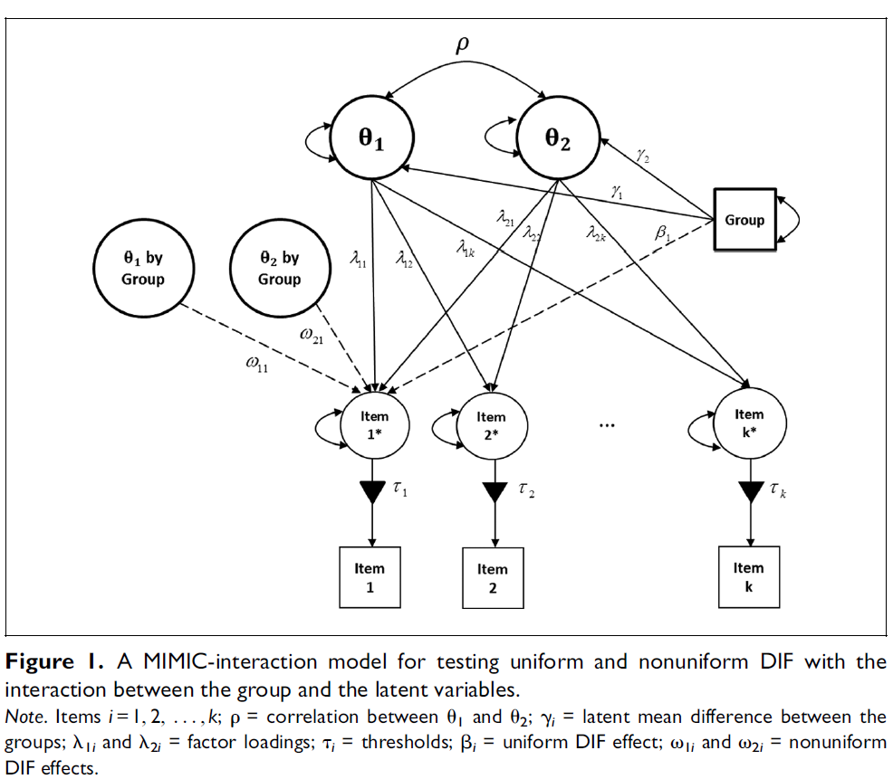
As Woods & Grimm (2011) noted, MIMIC can detect non-uniform DIF but IRT seems to perform better. This was later confirmed by Bulut & Suh (2017) who compared DIF statistics of the multidimensional extension of IRT-LRT, LR (with either observed or latent score matching) and MIMIC-interaction models under 2PL data. They found that the IRT largely outperformed both the LR and MIMIC in detecting non-uniform DIF and displayed the lowest FPs under all conditions, close to 0.05. LR and MIMIC had too low power for non-uniform DIF.

The inability of MIMIC to account for group differences in the variance of the latent factor (due to imposing equality constraints) impacts its type I error and power whenever the factor variance equality is violated. This was confirmed in the simulation studies of uniform DIF (Carroll, 2014) as well as non-uniform DIF (Harpole, 2015) despite purification procedures. It was further confirmed that MIMIC is riddled with inflated type I error if factor variance equality is violated even when the constant anchor or the sequential-free baseline as one of the best method of purification was used (Chun et al., 2016).

Yet another assumption is required. Simulation showed that all model fit indices testing for uniform DIF are insensitive to factor loading non-invariance (Kim et al., 2012). This indicates MIMIC should be used when loading invariance is achieved.

In the context of multidimensional test, Lee et al. (2017) evaluated the MIMIC with respect to type I error and power rates for uniform and non-uniform DIF. For type I error, the Benjamini-Hochberg procedure was used to decrease false positives. The simulations have varying parameters such as test length with number of DIFs, size of DIF, sample size differences between groups, correlation between the 2 latent traits and latent trait mean differences between groups. For uniform DIF (Table 3), type I error rates were close enough to the expected alpha value of 0.05. For non-uniform DIF (Figures 2-6), the power was low enough to warrant suspicions although this can be partially resolved by having greater test length.

Multilevel MIMIC was evaluated by comparing the Satorra-Bentler scaled likelihood ratio, AIC, BIC, SABIC as fit indices (Kim et al., 2015). In the context of loading non-invariance, all fit statistics had good power rates but only the BIC and SABIC performed well at controlling FP rates. In the context of intercept non-invariance, all fit statistics had good power rates but all perform badly at controlling FP rates when DIF size is large and only BIC had close to nominal rate for FP when DIF size is small. When the the S-B likelihood ratio was applied with Oort-adjusted χ² to control for model misspecification (i.e., the presence of non-invariant variable when the model assumes complete invariance by constructing a single model for both groups), therefore reducing FPs, not only the FPs were close to zero but the power was very high with respect to the intercept invariance. Son & Hong (2021) compared the Multilevel MIMIC and FMM under assumption of equal factor structure across levels. Both methods are reliable but, unlike FMM, the MIMIC had good power even with small cluster sample/size and regardless of unbalanced samples. Generally, factorial invariance and latent mean difference testing require at least N=50 clusters.

Bauer (2017) proposed the Moderated Nonlinear Factor Analysis (MNLFA) which combines the strengths of MGCFA and MIMIC, therefore addressing some of the above issues. Specifically, it allows group differences in variances, covariances and factor loadings but also accommodates multiple predictors, including discrete variables. MNFLA can behave like the standard MIMIC (or MIMIC-interaction) if we specify linear moderation of factor means and intercepts (or factor loadings). It can also reproduce the group differences in the variance-covariance parameters of the MGCFA by using a log-linear moderation. Another way to specify MNFLA as a MIMIC-type model is to add nonlinear constraints on loadings and variance-covariance parameters. Moderation functions for factor mean and variance can be implemented based on theory or empirical information, by simply including main effects, squared values and interactions. If criminality varies by gender and by age, the equation would be: gender + age + age^2 + gender*age + gender*age^2. This is what Bauer did in his analysis of the delinquency variables of the Add Health for which he found that MNLFA fits better than either MIMIC or MGCFA. More specifically, only MNLFA could detect that violent behavior becomes more variable across ages and that the correlations of these delinquency variables decreased across ages.

2.13. Third Generation DIF Analyses: Latent Class Analysis.

The 3rd-Gen DIF analysis, originally coined by Zumbo (2007), involving causal-search techniques such as LCA is akin to a factor analysis (FA) but at the group level. LCA is searching for clusters of item response probabilities while FA is searching for clusters of correlations between variables. Based on these patterns, latent groups (LCA) or latent variables (FA) are created. The basic idea in LCA is that DIF based on manifest, observable group variable (e.g., gender, race) may not be equivalent to DIF based on latent (i.e., unobserved) group variable. Cohen & Bolt (2005) were one of the first to prove it. Similarly, Chen & Jiao (2014) demonstrate that PISA scores exhibit DIF on items based on gender and social status that are inconsistent with DIF on items based on latent class. Their explanation is that DIF may be caused by manifest variables that are not included in the DIF analysis or by an interaction of multiple manifest grouping variables. LCA can detect heterogeneity and pattern within manifest groups. Indeed, a manifest within-group LCA can be conducted (Grover & Ercikan, 2017). But a more important research pertains to group differences, which can be assessed through various means, such as TCC plots (Hinton, 2015, p. 97) or factor score plots (Sawatzky et al., 2012, Figure 3) between the best fit class model and the one-class model or logistic regression with latent class as dependent and group as independent variable (Hinton, 2015). Although the major weakness of LCA is the over-extraction of classes, this can be alleviated through extensive exploratory analysis since one can inspect loadings and intercepts (Hinton, 2015, p. 94) or the number of persons in each class (Samuelsen, 2005, p. 62). Another difficulty is the interpretation of latent class variables as opposed to manifest variables as potential causes.

Class extraction can be decided upon through multiple means. Nylund et al. (2007) found BIC as well as Bootstrap LRT to be performing very well for class enumeration. BIC performed better than AIC and CAIC (both of which are not recommended) whereas BLRT performed better than the modified LRT of Lo-Mendell-Rubin that is designed to compare nested latent classes. For LCA modeling, either using categorical or continuous outcome variable, BLRT performs better than BIC. The class (or posterior) probabilities is another assessment of class model and represent the average probability of a person being assigned to a class. Good classification is achieved when diagonal elements are high and off-diagonal elements are low (Muthén & Muthén, 2000, Table 2). Entropy is another index widely used. A decision about cutoff is difficult however. Wang et al. (2017) reported that entropy >0.76 (or >0.84) is associated with 90% correct class assignment for a 3 (or 5) latent class model. They noticed that entropy is close to unity with small samples (N=50-100) and with more indicator variables (4 is bad but 8, 12, 20 indicators are good enough). Under conditions of N=500, 1000 or 3000, entropy values are largely below 0.90, but still slightly above 0.80 when latent class separation is large (Mahalanobis Distance=3).

As is true in IRT, LCA assumes local independence of indicator variables within classes. If ignored, over-extraction may happen. This can be examined through latent class proportions, with small class being probable evidence of spurious class. Furthermore, Asparouhov & Muthén (2011) proposed the Bayesian estimator which relaxes this assumption, given a correlation matrix estimated using an informative prior with mean zero but non-zero variance. They also argue that even if no over-extraction occurs the class proportions will be incorrect if local independence is ignored.

LCA has more potential in correctly identifying the DIF items as well as their causes. For instance, when Samuelsen (2005) analyzed data on an English language proficiency test, the LC approach displayed a pattern of DIFs related to one particular type of items (passage) whereas the MH method failed to detect it. LCA was justified by the findings 1) that DIFs detected by MH was a small subset of LCA and 2) that correct detection rates decreased as within group heterogeneity increases and decreased further as DIF sizes increase. Since a manifest group doesn’t capture heterogeneity so well it could be that, instead of reflecting the difference in the majority of the two manifest groups, the observed bias reflects difference in small subsets of each group (Samuelsen, 2005, p.78).

The LCA procedure is possible with LR, as proposed by Zumbo et al. (2015, Figure 2). In step 1, the usual LR model for DIF is applied. In step 2, the class enumeration is achieved through likelihood ratio test and other information criteria like BIC and AIC. In step 3, regression with one predictor is performed for each theoretically relevant predictor of class membership. In step 4, all significant predictors are entered altogether in the LR regression with class as dependent variable. But Zumbo relied too much on significance tests. One must proceed further, as Hinton (2015) did.

Another advantage of latent-based DIF methods is to account for item parameter drift (IPD) which reflects the deviation of item parameters from their true values due to its successive testing administrations (Park et al., 2016). Such lack of invariance over time can be captured by latent classes. But when ignored, examinee ability is impacted.

LCA can be extended using multilevel approach. The most appropriate method to detect the correct number of levels is to use model fit indices. Sen et al. (2019, p. 277) compared the performance of AIC, BIC, CAIC and SABIC. It was found that BIC and CAIC tended to select the correct model more often as opposed to SABIC and AIC, with AIC performing the worst. Similarly, Lee et al. (2018) simulated clustered data with large cluster size and found that BIC correctly selected the multilevel model often unlike the AIC.

LCA is now highly regarded. But guessing, as noted earlier, can invalidate estimations if not modeled. One method to deal with this issue is the Mixture IRT (MixIRT) model (Cohen & Bolt, 2005) which can be developed into Multilevel MixIRT (MMixIRT) as proposed by Cho & Cohen (2010). MixIRT is simply the latent class version of IRT. Raykov & Marcoulides (2020) raised the issue that a sizeable guessing parameter estimate, which would not reflect guessing processes, may emerge owing to heterogeneous populations consisting of several unobserved subpopulations. In this case, Mixture IRT seems to be the ideal method due to capturing latent classes.

Unfortunately, DeMars & Lau (2011) questioned the viability of MixIRT as a method of DIF. Simulation fails to recover well the true class membership used to generate the data. Both the discrimination and difficulty parameters were biased and the direction depended on whether there was group impact. DIF sizes were overestimated when there is no impact. MixIRT performs generally better when DIFs are plentiful, which then is contradictory with the concept of DIF being a disturbance if now the DIF is a major phenomenon. This pattern is not seen in traditional methods of DIF. Furthermore, if a large % of items show DIF, it makes no sense to match examinees on ability because the test would measure two disparate constructs. Remember that greater numbers of DIF items will erode power and increase the Type I error rate (Finch, 2005; Wang & Yeh, 2003). Finally, MixIRT likely will perform less well in contexts where each source of DIF affected only a small number of items. Despite recognizing the limitations of MixIRT, Sawatzky et al. (2016) showed that this method performs better than traditional IRT due to accounting for population heterogeneity.

3. Analysis of the GSS Wordsum test.

The GSS subset data, R codes and full results are all available here.

3.1. Method.

The survey data is available at the GSS website, with the relevant codebook. The Wordsum is the sum of the following 10 questionnaires/items. Needless to say, these questions are overly culturally loaded.

A. SPACE 1. school 2. noon 3. captain 4. room 5. board 6. don’t know
B. BROADEN 1. efface 2. make level 3. elapse 4. embroider 5. widen 6. don’t know
C. EMANATE 1. populate 2. free 3. prominent 4. rival 5. come 6. don’t know
D. EDIBLE 1. auspicious 2. eligible 3. fit to eat 4. sagacious 5. able to speak 6. don’t know
E. ANIMOSITY 1. hatred 2. animation 3. disobedience 4. diversity 5. friendship 6. don’t know
F. PACT 1. puissance 2. remonstrance 3. agreement 4. skillet 5. pressure 6. don’t know
G. CLOISTERED 1. miniature 2. bunched 3. arched 4. malady 5. secluded 6. don’t know
H. CAPRICE 1. value 2. a star 3. grimace 4. whim 5. inducement 6. don’t know
I. ACCUSTOM 1. disappoint 2. customary 3. encounter 4. get used to 5. business 6. don’t know
J. ALLUSION 1. reference 2. dream 3. eulogy 4. illusion 5. aria 6. don’t know

According to Wolfle (1980, p. 110), its correlation with the Army General Classification Test (AGCT) is 0.71. The test reliability was 0.63 for blacks and 0.71 for whites (Hu, 2017).

Before examining the items, I analyzed the responses. Only 460 GSS respondents (3.7%) refused to answer any of the WORDSUM items, and we ignored them throughout the analysis. The refusals completed fewer years of schooling (x = 10.5 vs. 12.9 years), but were also more variable in schooling (s = 3.6 vs. 2.8 years). I considered whether item nonresponses — other than complete refusal — should be treated as incorrect answers. I compared the internal consistency reliabilities among complete responses and among incomplete responses, treating nonresponses in the latter group as errors. These were virtually the same, 0.62 and 0.64. Further, the correlations between educational attainment and WORDSUM among the complete and incomplete responses were identical. Thus, I assumed that item-specific nonresponses were erroneous responses.

Missing values are denoted as IAP (inapplicable) for -1, and NA (not answered) for 9. Values of 0 and 1 are the incorrect and correct answers. The value of 9 should be recoded as 0, for incorrect answers.

3.2. IRT: Results.

First of all, unidimensionality must be checked using parallel analysis. I use the random.polychor.pa function which estimates polychoric correlation, a more appropriate approach for dichotomous variables. For each group, there was 1 dominant factor, with the second factor in both case being much less important than the first factor and having eigenvalue less than 1.

Using mirt package, ICC plots are computed based on the unconstrained (i.e., free) 3PL model and without applying purification. Except for word E, all items are biased. As we will see later, this is misleading.

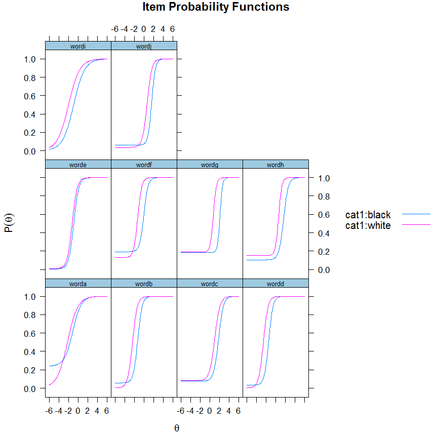
First step is to estimate the baseline model in which the item parameters (a and b) are set to be equal across groups while allowing latent means and variances differences. This baseline serves as a basis for checking anchor items for linking the two groups on the same metric before applying the real IRT method of DIF.

The DIF() function uses scheme = ‘drop’ which is a sequential DIF anchor method that drops the constraints for one item at a time while leaving all others with constraints. The program runs these models and see which ones fit the data best. The following command, by allowing the estimation of a and b parameters, simultaneously considers both types of DIF.

> (DIFboth<- DIF(baseline, which.par=c('a1', 'd'), scheme='drop', seq_stat=.05))
      converged     AIC   SABIC      HQ     BIC     X2 df     p							
worda      TRUE  -0.751   8.537   4.387  14.893  4.751  2 0.093							
wordb      TRUE   2.897  12.185   8.035  18.541  1.103  2 0.576							
wordc      TRUE  -3.512   5.776   1.627  12.132  7.512  2 0.023							
wordd      TRUE   3.599  12.887   8.737  19.243  0.401  2 0.818							
worde      TRUE -89.727 -80.438 -84.588 -74.083 93.727  2     0							
wordf      TRUE -16.838  -7.550 -11.700  -1.194 20.838  2     0							
wordg      TRUE -29.861 -20.572 -24.722 -14.217 33.861  2     0							
wordh      TRUE   0.368   9.656   5.506  16.012  3.632  2 0.163							
wordi      TRUE   3.508  12.796   8.646  19.152  0.492  2 0.782							
wordj      TRUE   2.364  11.652   7.502  18.008  1.636  2 0.441

As can be seen, 2 items stick out like a sore thumb when considering only model fit indices: Word E and G. While Word F displays much higher AIC than most items, the BIC was smaller. I included F in the studied DIFs because there was no clear indication of no DIF. The p-values are too sensitive to sample size and I wouldn’t recommend focusing on it. For instance, Word C is significant (p=0.023) but displays fit index values similar or even lower than other items which are non-significant. It is probably safe to assume C is not biased. The following table displays the parameter estimates for the biased items. It is interesting to note the wide CIs for the 0.05 level in Word F and G for the black group. The a and b parameters are not estimated with accuracy.

# Black a-b-c-parameters		# White a-b-c-parameters

$worde		                        $worde
           a1     d g  u		           a1     d g  u
par     1.916 1.771 0  1		par     1.939 0.567 0  1
CI_2.5  1.656 1.586 0 NA		CI_2.5  1.789 0.442 0 NA
CI_97.5 2.175 1.957 1 NA		CI_97.5 2.089 0.693 1 NA

$wordf		                        $wordf
           a1      d     g  u		           a1     d     g  u
par     2.371  0.078 0.194  1		par     2.418 0.844 0.130  1
CI_2.5  1.501 -0.329 0.118 NA		CI_2.5  2.132 0.593 0.065 NA
CI_97.5 3.240  0.485 0.301 NA		CI_97.5 2.704 1.094 0.242 NA

$wordg		                        $wordg
            a1       d     g  u		           a1      d     g  u
par      5.736 -11.605 0.185  1		par     3.207 -5.315 0.189  1
CI_2.5  -1.780 -26.036 0.169 NA		CI_2.5  2.735 -6.120 0.173 NA
CI_97.5 13.252   2.826 0.202 NA		CI_97.5 3.678 -4.511 0.205 NA

After confirming these DIFs with the baseline, a restricted model in which all items except E, F, G are anchored is fit to the data. Effect size estimates and plots are produced from the restricted model. Effect size plots are displayed below. First plot, using Meade’s (2010) IDS, we see that only E and G display large DIF, while F displays small DIF. Word E favors blacks at low levels of ability while G favors whites at high levels of ability. Other items display only one curve because of equality constraints. Second plot, using Chalmers’ (2018, 2022) DRF, which is probably the most accurate effect size measure, we see that word E favors blacks at the middle level and G strongly favors whites at the high level. Third plot, based on Chalmers again, shows the DTF plot or the expected latent score. There is no meaningful impact against either group.

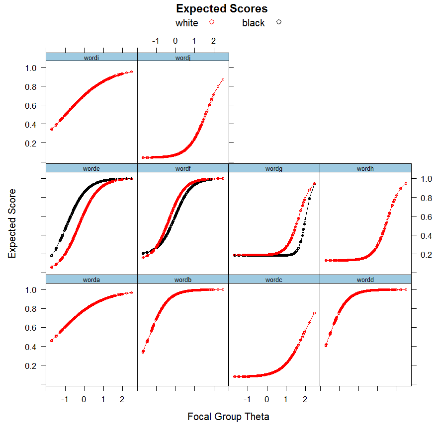
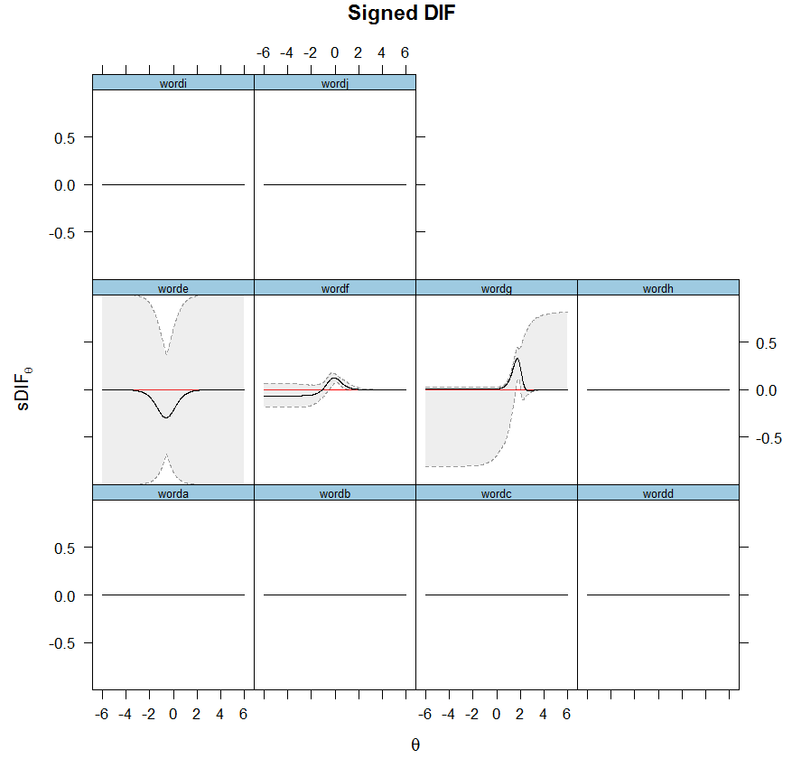
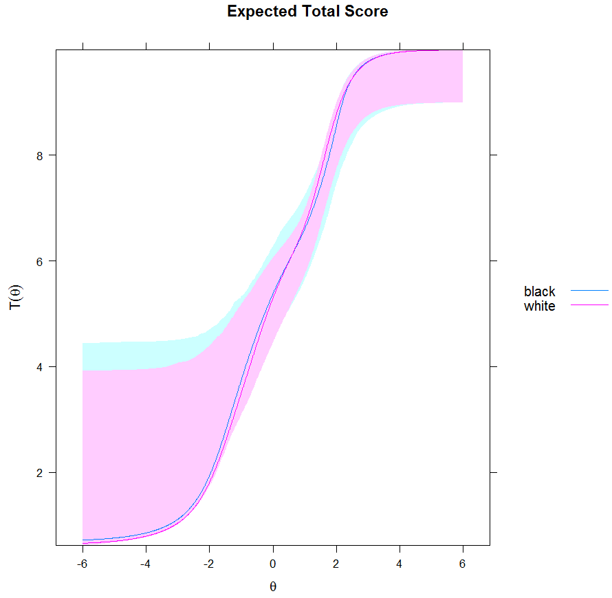
The problem with the above plots as well as DIF size estimates comes from the wide confidence intervals (CIs). A possible reason is that the c-parameter is poorly estimated, producing large standard errors (Hambleton et al., 1991, p. 112). Ideally, we always want to investigate the 3PL model. But the CIs are so large that I’m now reporting the results from 2PL as well. In short, the same items in the baseline model were detected as DIF but the relative fit indices and effect sizes are different. Below, the effect size plots are displayed for the 2PL model. Except for word G, the same pattern is observed.

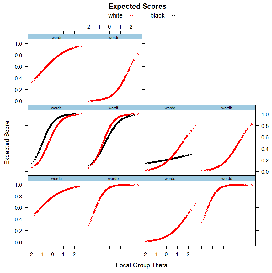
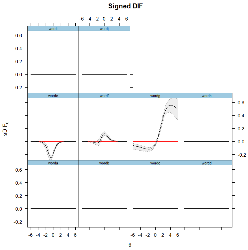
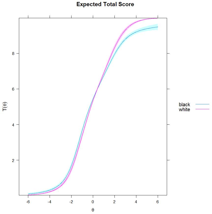
The present analysis is unweighted. Yet it is very important to apply sampling weight, since it affects parameter estimates, standard errors and model fit. When I applied the weights, the curves and estimates of the baseline models were similar. However, when attempting DIF detection the fit indices were identical across all items. Whatever the cause, this outcome cannot be trusted.

3.3. Multilevel LCA: Results.

LCA is performed using glca package. I specify the multilevel structure similar to what I have done in my 2017 analysis of the black-white gap over time by using age centered and its square as fixed effects while using a group cohort variable (21 categories) as random effects. As explained in my 2017 paper, the reason for including age is because cohort and age are correlated and normal regression will not accurately separate both effects. Survey weight option is not available in glca.

Class enumeration is achieved the traditional way without any fixed or random effects variables, comparing 2-class, 3-class, and 4-class models. The BIC index value selects the 4-class model whereas the entropy selects the 3-class. I looked at the class-conditional item probabilities for the 4-class model and two classes exhibit a similar pattern of probabilities, which suggests a spurious class was extracted.

Below I display the correct response probabilities for the 3-class model and it looks obvious that class 3 is recognized as the high ability class, and class 1 the medium ability class due to having higher probability of correct response than class 2, the low ability class. While class 3 exhibits high % of correct answer in all items, class 1 has low % in word C, G, H, J, and class 2 has low % in word C, E, F, G, H, J. Finally, noticed that class 1 has high population proportion, especially compared to class 2.

Item-response probabilities (Y = 2) :										
        d$worda d$wordb d$wordc d$wordd d$worde d$wordf d$wordg d$wordh d$wordi d$wordj										
Class 1  0.8470  0.9826  0.1528  0.9887  0.8311  0.8550  0.2110  0.2132  0.7959  0.1323										
Class 2  0.5513  0.6115  0.0893  0.6826  0.2591  0.3276  0.2151  0.1289  0.4485  0.0499										
Class 3  0.9568  0.9939  0.5908  0.9943  0.9806  0.9963  0.7469  0.8090  0.9267  0.6917

Performing multilevel LCA, I closely follow the procedure in the Introduction to glca package by comparing nested models, each step specifying a different constraint. First step was to compare these 3 models: no cohort random effects 3-class model, 3-class model with cohort non-invariant probabilities, 3-class model with cohort invariant probabilities. The last model has better fit. Adding random effects indeed improved the model. The pattern of item probabilities when accounting for random cohorts is very similar to the above table.

After establishing invariance across cohorts, two models were compared: 3-class cohort invariance with age invariance across cohorts against age non-invariance across cohorts. The fit indices indicate that age effects were invariant across cohorts. Finally, when the black-white variable was added to this model, there was substantial improvement in fit. This means race was closely related to the class membership. Furthermore, when the non-invariance was assumed for all level-1 variables the model fit deteriorated. Although this suggests that race effect was invariant across cohorts, the decrease in fit could be due to age non-invariance being misspecified.

For this reason, in the model with non-invariance level-1 slopes, I examine the across-cohort Odds Ratios of class membership for the black-white variable, as coded 0/1 indicating that whites have higher (or lower) probability of class membership than blacks if OR is higher (or lower) than 1. On average, the ORs in Class 2/3 (low/high ability) are ranged between 0.20 and 0.30. Here are the ORs for Class 1/3 (medium/high ability) across successive group cohorts: 9.91, 8.75, 3.37, 4.05, 5.83, 3.90, 7.39, 4.15, 4.17, 6.25, 9.00, 4.49, 13.77, 5.46, 6.33, 6.87, 8.60, 5.84, 5.94, 233.03, 28.17. There is a wide variation across cohorts for the Class 1/3 but no trend in the ORs across cohorts. Overall, it seems that whites have more probabilities of belonging to either the low or high ability class.

Although it is possible to model latent clusters across the level-2 variable (i.e., cohorts), it wouldn’t improve its meaning. More importantly is that the above analysis is mainly exploratory. No R packages seem available right now to directly detect DIF across latent groups in the same way as IRT by estimating parameter difficulty while applying purification or even modeling guessing. On the other hand, WinBUGS and Mplus provide a more complete DIF test with LCA.

4. Discussion.

In this study, I showed that only 2 items display substantial bias, one favors blacks, one favors whites. The impact on the latent total score is small. It seems rather surprising that a culture loaded test such as wordsum is not biased against lower scoring groups (i.e., blacks). Relying either on 2PL or 3PL model, Word E and G reveal themselves as DIF. What about the cause of DIF? Word G is only biased against blacks at high levels of ability. LCA shows actually that only the high ability class has a high correct response rate of 74% while both the low and medium ability class have a correct response rate of 21%. Specialized words are most likely being answered right by high ability persons. Word E favors blacks at the medium (or low) level depending on Chalmers (or Meade) effect size. LCA reveals that word E is answered correctly by most people in medium and high ability class (83% and 98%) but not by low ability class (26%).

One obvious limitation with the present analysis, as is also the case with all other DIF analyses you see everywhere is that the DIF screen is internal. As noted by Shih & Wang (2009) this is a problem because to detect DIFs in the first step of the purification procedure, you want the items to be free of DIF. It has been sometimes suggested that the initial DIF screening must be based on theory, prior knowledge or expertise. This procedure is more feasible for a cognitive test that has been widely and repeatedly administered and studied by psychologists.

One important question as for DIF methods is whether one should use manifest or latent variable approach. DeMars & Lau (2011) showed the limitations of LCA yet it cannot be denied that heterogeneity is a concern. Latent variable starts with an exploratory approach while manifest variable starts with a confirmatory approach. It is often suggested that a latent class regression must be performed using manifest variables suspected being the source of DIF. Thus LCA may provide additional informations. However the classes are not clearly defined when the predictors fail to account for a substantial variation of the class membership. This situation does not help our understanding of DIF and is only interesting from a statistical perspective. Since IRT always hits the mark with respect to inferences, IRT should remain the main method of DIF. Unlike LCA, IRT easily accounts for guessing and purification.

Richwine (2009) in his study of PIAT-Math has written about the limitation of DIF testing methods: “Like all internal validity checks, it can detect only bias that varies from item to item. If there were a uniform bias affecting every item identically, SIBTEST would not see it. This could be a problem on a test of immigrant verbal skills, where lack of English knowledge could conceivably push down immigrant scores compared to native scores, even as the relative difficulty of each item remains the same for both groups. However, this is far less likely on a math test, in which the verbal content of an item is unrelated to the difficulty of the mathematical concept being tested. When language bias affects a math test, its impact will almost certainly vary by item.” (pp. 53-54). Fortunately, a combination of methods, with IRT at the item level, with MGCFA at the subtest level, will improve test bias overall.

A general improvement of test bias, especially in an IRT framework, is the promising approach of Computerized Adaptive Testing (Hambleton et al., 1991, ch. 9). Lord during the 1960s began a comprehensive research and concluded that a fixed-test length, as is common in test administration, is inefficient for comparing low and high ability groups. A test can be shortened without any loss of measurement precision if the items actually matched the examinee ability. In CAT, the sequence of items administered depends on the examinee’s performance on earlier items in the test. Such procedure definitely helps DIF methods in producing even more accurate results.

Recommended readings.

Asparouhov, T., & Muthén, B. (2011, July). Using Bayesian priors for more flexible latent class analysis. In proceedings of the 2011 joint statistical meeting, Miami Beach, FL. American Statistical Association Alexandria, VA.
Bauer, D. J. (2017). A more general model for testing measurement invariance and differential item functioning. Psychological methods, 22(3), 507.
Beretvas, S. N., & Walker, C. M. (2012). Distinguishing differential testlet functioning from differential bundle functioning using the multilevel measurement model. Educational and Psychological Measurement, 72(2), 200-223.
Chalmers, R. P. (2022). A Unified Comparison of IRT‐Based Effect Sizes for DIF Investigations. Journal of Educational Measurement.
Cho, S. J., & Cohen, A. S. (2010). A multilevel mixture IRT model with an application to DIF. Journal of Educational and Behavioral Statistics, 35(3), 336-370.
DeMars, C. E. (2009). Modification of the Mantel-Haenszel and logistic regression DIF procedures to incorporate the SIBTEST regression correction. Journal of Educational and Behavioral Statistics, 34(2), 149-170.
DeMars, C. E. (2011). An analytic comparison of effect sizes for differential item functioning. Applied Measurement in Education, 24(3), 189-209.
DeMars, C. E., & Lau, A. (2011). Differential item functioning detection with latent classes: how accurately can we detect who is responding differentially?. Educational and Psychological Measurement, 71(4), 597-616.
Finch, H. (2005). The MIMIC model as a method for detecting DIF: Comparison with Mantel-Haenszel, SIBTEST, and the IRT likelihood ratio. Applied Psychological Measurement, 29(4), 278-295.
Finch, W. H., & French, B. F. (2008). Anomalous type I error rates for identifying one type of differential item functioning in the presence of the other. Educational and Psychological Measurement, 68(5), 742-759.
Finch, W. H., & French, B. F. (2014). The impact of group pseudo-guessing parameter differences on the detection of uniform and nonuniform DIF. Psychological Test and Assessment Modeling, 56(1), 25.
Hambleton, R. K., Swaminathan, H., & Rogers, H. J. (1991). Fundamentals of item response theory (Vol. 2). Sage.
Hinton, D. (2015). Uncovering the root cause of ethnic differences in ability testing: differential test functioning, test familiarity and trait optimism as explanations of ethnic group differences (Doctoral dissertation, Aston University).
Jiao, H. (2022). Comparison of different approaches to dealing with guessing in Rasch modeling. Psychological Test and Assessment Modeling, 64(1), 65-86.
Li, Y., Brooks, G. P., & Johanson, G. A. (2012). Item discrimination and Type I error in the detection of differential item functioning. Educational and Psychological Measurement, 72(5), 847-861.
Linn, R. L., Levine, M. V., Hastings, C. N., & Wardrop, J. L. (1981). Item bias in a test of reading comprehension. Applied psychological measurement, 5(2), 159-173.
Oliveri, M. E., Olson, B., Ercikan, K., & Zumbo, B. D. (2012). Methodologies for investigating item- and test-level measurement equivalence in international large-scale assessments. International Journal of Testing, 12(3), 203-223.
Park, Y. S., Lee, Y. S., & Xing, K. (2016). Investigating the impact of item parameter drift for item response theory models with mixture distributions. Frontiers in Psychology, 7, 255.
Roznowski, M., & Reith, J. (1999). Examining the measurement quality of tests containing differentially functioning items: Do biased items result in poor measurement? Educational and Psychological Measurement, 59, 248-269.
Wang, W. C., & Yeh, Y. L. (2003). Effects of anchor item methods on differential item functioning detection with the likelihood ratio test. Applied Psychological Measurement, 27(6), 479-498.

DIF Review and Analysis of Racial Bias in Wordsum Test using IRT and LCA

1. The complexity of DIF detection.

1.1. Item Characteristic Curve.

1.2. The A-B-C-parameters.

1.3. Matching for total score with measurement error and bias.

2. Statistical procedures.

2.1. ANalysis Of VAriance (ANOVA).

2.2. Transformed Item Difficulty, or Item Correlation Method.

2.3. Partial Correlation Index.

2.4. Chi-Square (χ²).

2.5. Expert Judgment.

2.6. Standardization P-DIF method.

2.7. Logistic Regression (LR).

2.8. Mantel-Haenszel (MH).

2.9. Simultaneous Item Bias (SIBTEST).

2.10. Item Response Theory (IRT).

2.11. Means And Covariance Structure (MACS).

2.12. Multiple Indicators Multiple Causes (MIMIC).

2.13. Third Generation DIF Analyses: Latent Class Analysis.

3. Analysis of the GSS Wordsum test.

3.1. Method.

3.2. IRT: Results.

3.3. Multilevel LCA: Results.

4. Discussion.

Related

Leave a Reply Cancel reply

Recent Posts

Categories

Data Analysis

Databloggers

Journals

Library

Archives

Meta

DIF Review and Analysis of Racial Bias in Wordsum Test using IRT and LCA

1. The complexity of DIF detection.

1.1. Item Characteristic Curve.

1.2. The A-B-C-parameters.

1.3. Matching for total score with measurement error and bias.

2. Statistical procedures.

2.1. ANalysis Of VAriance (ANOVA).

2.2. Transformed Item Difficulty, or Item Correlation Method.

2.3. Partial Correlation Index.

2.4. Chi-Square (χ²).

2.5. Expert Judgment.

2.6. Standardization P-DIF method.

2.7. Logistic Regression (LR).

2.8. Mantel-Haenszel (MH).

2.9. Simultaneous Item Bias (SIBTEST).

2.10. Item Response Theory (IRT).

2.11. Means And Covariance Structure (MACS).

2.12. Multiple Indicators Multiple Causes (MIMIC).

2.13. Third Generation DIF Analyses: Latent Class Analysis.

3. Analysis of the GSS Wordsum test.

3.1. Method.

3.2. IRT: Results.

3.3. Multilevel LCA: Results.

4. Discussion.

Share this:

Related

Leave a Reply Cancel reply

Recent Posts

Categories

Data Analysis

Databloggers

Journals

Library

Archives

Meta