Back in 2014 I wrote an extensive review of studies on the income mobility rate over time and across countries and discussed whether it truly fits the Great Gatsby Curve, a term based on the observation of the negative relationship between mobility and inequality, that is considered by many as unfair because it implies that higher inequality causes lower mobility. However I did not consider Black-White difference in mobility. Because mobility and inequality are interrelated, I will cover both topics here. Three findings are worth noting: 1) IQ explains a very large share of the BW mobility gap, 2), the Civil Right did not improve the Blacks’ outcomes 3) the Black Migration aggravated the Blacks’ social outcomes.
CONTENT
Increasing Income Inequality and Black-White Gap
Re-Analysis of the Wage Gap in the NLSY79/97
Mobility Trends and Black-White Gaps
Increasing Income Inequality and Black-White Gap
The trend of the gap over time is probably the most important research. Daly et al. (2017) informed us that in the CPS data the BW wage gap increased between 1979 and 2016 in the U.S. for both men and women. Generally Black men earn 20% less than White men and Black women 5% less than White women. One interesting finding is the decomposition of the BW gap obtained by a regression. Control variables include: State of residence, education, part-time job, industry/occupation and age. And then we are left with the last component: The unexplained variance. And this one is not only very large but increasing over time.
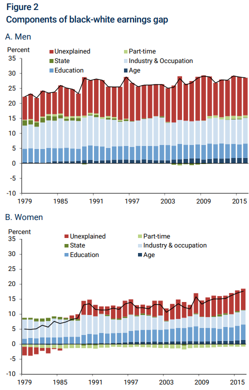
Economists want us to believe schooling is the best chance equalizer. The typical argument is that returns to education increased substantially over time along with inequality in education (Bloome et al., 2018). Yet this returns effect is only visible in the BW women gap and does not account for the unexplained. Furthermore, we must know that education attainment is likely caused by IQ (Jensen, 1973) with not much evidence that education causes IQ (Lasker & Kirkegaard, 2022). Herrnstein & Murray (1994, pp. 511, 541-542) informed us that IQ outdoes education in almost everything and that technology and complexity created more jobs for the cognitive elite and caused more reliance on intelligence in everyday life, a view shared and explained by Gottfredson (2003). That IQ outdoes education in a regression equation is important because as Strenze (2007) cogently noted, when comparing IQ and parent SES, a lower coefficient for IQ would have indicated it was a mere byproduct of the causal effect of SES. Because IQ is stronger than either parent SES or educational attainment, it gives more weight to the hypothesis that IQ was the causal factor. Although this is merely suggestive and doesn’t prove anything, it adds weight (albeit a little) to the results from natural experiments.
Later, Daly et al. (2020) showed (Figure 2) that the increase in education levels does not moderate further the wage gap for either Black men or women and this holds true across all cohorts from 1979 to 2002.
The evidence suggests that income varies considerably within education levels. Cheng et al. (2019, Figures 3-5) analyzed the trajectories of the BW earnings gap among men between 24 and 46 years-old and across three cohorts (1945-1954, 1955-1964, 1965-1974) in the U.S. by using the SIPP-SSA data set. The result from growth curves splitted by education levels shows that among less than high school men, Blacks earnings declined substantially relative to Whites across cohorts. However, among college graduates, the gap also widened over time. Further examination revealed that while Black and White college graduates have the same proportions of business majors, the proportion of high-paying majors (STEM, law and medicine) is substantially greater for Whites. Not only that, but among college graduate men, Whites are also more likely to obtain a doctorate degree. Finally, among middle-tier education groups, the gap widened and then narrowed a little bit. In this data the driving force of the widening gap is to be found among less educated and very highly educated men. This economic polarization supports the main idea of The Bell Curve in chapter 15.
Ren (2022a) provides further evidence of this huge income variance. After analyzing the BW earnings gap and growth in the PSID, using a regression including many covariates, he found that less educated Black men start with more disadvantaged earnings which then stay constant over time while college graduated Black men start with less disadvantaged earnings which then grow over time. The first finding is that education mitigates the initial gap (i.e., at early-career stage) by reducing or removing information asymmetry about the worker’s productivity. The second is that college graduated Black men are facing increased, fierce competition which causes them to lose ground over time. Such evidence is given by the examination of the 97th percentile of income distribution comprising 75% of White college graduates compared to 30% in the unrestricted sample.
Subsequently, Ren (2022b) focuses on the BW gap at early-career stage. But why early career? The rationale is for better capturing the impact of human capital (IQ, education, etc.) on income and potential stereotype effects because credentials likely play a much more salient role for Black men as “productivity signal” and because wage gaps developed during career growth can be explained by occupational tracks and workplace dynamics as shown earlier. The predicted Black-White men earnings gap, based on a multiple regression using the entire sample of the PSID, declines substantially as education levels increase (from 54.8% for high-school to 3.8% for Graduate). Then he examines the impact of race-education interaction across cohorts by inserting cohort, race x education and race x education x cohort in a regression. Cohort 1 (1968-1981) includes those who entered labor markets immediately after the Civil-Rights Movement. Cohort 2 (1982-1993), used as reference category, includes labor markets during the conservative period of Reagan and George H.W. Bush. Cohort 3 (1994-2001) includes labor markets during the economic boom under Clinton. Cohort 4 (2002-2007) and Cohort 5 (2008-2014) are labor markets during the pre- and post-Great Recession era. For Cohorts 1, 3, 4, and 5 we get the following coefficients of the race x education x cohort interaction: 0.41, 0.21, 0.25, 0.29. Thus, after Cohort 2, it appears that education becomes slightly more important for Black men over time during early-career stage. But because pooling all respondents runs the risk of confounding era-specific dynamics of the labor market, Ren broke the sample into sub-samples and re-estimated the model separately for each cohort. The conclusion is unchanged. Finally, Ren has an interesting comment on the NLSY79. Its cohort corresponds to the 1980s period under which the economic situation of Blacks suffered particularly, which means between-group comparison of income should be supplied with more data from other periods.
So far we haven’t discussed adjustment for IQ, right? When looking across 3 time periods using the NLS-OC, NLSY79 and NLSY97, Thompson (2021) found that returns to highest grade completed becomes stronger over time, that the returns to IQ becomes a lot stronger than education over time, and that the returns to IQ is overall stronger for Blacks but also becomes increasingly larger for Blacks than for Whites over time. Unsurprisingly the effect of either education or IQ becomes increasingly stronger at reducing the wage gap among men over time. Two limitations are reported. Firstly, the standardized test scores of the old NLS-OC were of lower quality as these tests were not administered by the NLS survey enumerators but by high schools and they involved more than 30 different standardized tests, and were measured with substantial error or were largely different from those available in the later surveys. Fortunately the NLSY79 survey collected such test scores in the 1980 and a comparison with the AFQT shows little difference in the coefficients of the earnings equations. Secondly, the NLS-OC probably missed respondents whose education did not advance beyond primary school. A robustness check by truncating the data in the same way for both the NLSY79 ad NLSY97 confirmed the main findings.
The real problem with Thompson however concerns the estimates. The model, which includes persons with zero earnings, incorporates both education and IQ but accounts for only 9.8%, 16.3% and 28.1% of the gap when using the inverse hyperbolic sine of earnings, yet 31.2%, 44.4%, and 37% of the gap when using log of hourly wages and excluding zero earnings. It is only when using the first (likely erroneous) approach that we see human capital becoming increasingly more important across successive cohorts but at the same time disappointing as to their predictive power. Obviously, a single-year measure was used but this cannot account for such low percentages. If the inclusion of zero earnings is the main explanation, that is quite surprising. Another surprising detail is the sample size about 10 or 20 times larger than most other published papers on the NLSY.
How do other studies compare to Thompson? For instance, when O’Neill et al. (2006) analyzed the NLSY79, including AFQT only in the regression reduces the wage gap by 73% among men with no zero earnings. Two problems. The use of a single-year income measure. No usage of sampling weights. So the analytic sample is not necessarily representative of the U.S. population. O’Neill was an extension and replication of Johnson & Neal (1998, Table 14-5) who reported that AFQT correlates stronger with earnings among Black men than among White men and that only controlling for AFQT cuts the gap in half. Wages averaged over 1990-1992, no zeros, no sampling weights. Cavallo et al. (1997, Table 9.6) also analyzed the NLSY79, and found that AFQT, parent SES, education, experience explain 38%, 18%, 17% and 19% respectively. The effect of AFQT likely was moderated by SES but it still reduces the wage gap by 38%. They used a single year income measure, excluded earnings below $5000 and used sampling weights.
Re-Analysis of the Wage Gap in the NLSY79/97
What a mess! For this reason, I decided to run my own analysis of the NLSY79/97. In these data, I separately analyze annual income and hourly wage variables, both averaged across 10 years so as to reduce measurement error. Another advantage of averaging is that if you still notice someone having zero earnings it means this person is likely out of the labor force and not seeking a job rather than just temporarily unemployed. Something you cannot see when using a single-year measure. This prevents the inclusion of the “wrong” people in the study sample. Years of self-reported earnings are selected in such a way that the mean age of male respondents falls between 30 and 40 years, with a 33 years-old average for both cohorts to make them comparable. Unlike previous researchers, I not only use the observed AFQT/ASVAB score but also their factor score derived from factor analysis because the g factor is the core ingredient of cognitive tests. Another factor usually unaccounted for is the interaction of race and IQ which, assuming strong interaction favoring Blacks, may reveal an otherwise stronger effect of IQ. I finally use the NLSY custom weights (NLSY79) (NLSY97) in accordance with the years of the data that I use (e.g., if I include variables for the years 1979, 1991, 1992, and 2000, then I request a weight for the selected years). Income variable (in constant dollars) is log transformed. Race variable (BW) is coded as 0=Black 1=White. The data (here) and SPSS syntax and full results are available (here). Tables below display regression coefficients for the equation with factor score. All coefficients are significant (p<0.001) except those italicized (p>0.050).
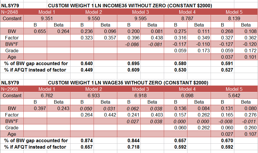
In the NLSY79, Model 2, the general factor alone accounts for 64% or 87% depending on whether the outcome is annual income or hourly wage. It is way stronger than AFQT for which numbers are 45% and 66%. Adding the interaction of IQ with race in Model 3 changes everything however. The interaction for the factor score is either weak or non-existent but such an effect is very strong for the observed score. This means that when cognitive ability increases, the non-g factor becomes more important in accounting for the BW wage gap but the g factor score is still the dominant variable. The most striking result is observed in Model 4. After the inclusion of education, the wage gap increased substantially. How to interpret this? Once Blacks and Whites are adjusted for IQ, Blacks actually had higher education, which means after controlling for education the Black advantage in education on earnings is removed.
Surprising but true. If you play with my data and codes, you can directly confirm this in one regression with Grade as dependent variable and BW along with Factor score as independent variables. The sign of BW starts positive but becomes strongly negative once Factor is added, and because I coded White as higher value, it means that White men achieve lower education than Black men when they have similar IQ.
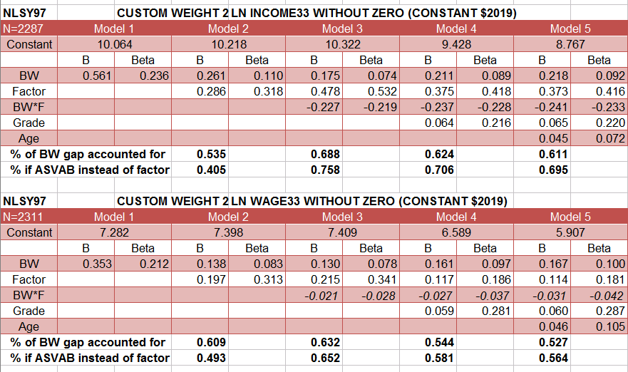
Now in the NLSY97, we observe a similar pattern. The effect of the general factor alone accounts for 53% and 61% of the annual income and hourly wage gap, while the respective numbers for ASVAB are 40% and 49%. However here, the interaction of race and IQ is much stronger than in the earlier cohort. The gap reduces substantially for ASVAB*race interaction, accounting for 76% (income) and 65% (wage). This indicates that IQ reduced substantially the wage gap among high IQ men in more recent cohorts. On the other hand, the interaction of race with the general factor is only strong in the income equation (B=-0.227). Generally the observed score is more impactful than the factor score in reducing the wage gap, as seen in Model 3, meaning that non-g factor increased in importance relative to the g factor across cohorts.
A curious pattern can be observed in both cohorts. When I use annual income as a dependent variable, the independent effect of g scores on income is much stronger than education but that isn’t true at all when hourly wage is the dependent variable.
How do my results compare with Thompson’s much larger sample? For the NLSY79, he explained in the footnote that his estimates were indeed smaller than reported by Johnson & Neal (1998) but he admitted that if he restricted the sample to cohorts born after 1961 and included only IQ, the wage gap would reduce by 58%. But a more likely and general cause regarding the three cohorts could be, as Thompson suspects, the inclusion of zero earnings in his preliminary analysis. Finally, looking at my result, one might even be reminded of Nyborg and Jensen (2001).
Mobility Trends and Black-White Gaps
Mobility isn’t easy to measure well. One has to account for lifecycle bias. Chetty et al. (2014a, 2014b) showed that estimates stabilize after (or around) age 30 for both parents and children measurements. One also has to correct for measurement error of single-year income by simply averaging across years and producing an accurate measure of permanent income, with the ideal age around which centering must be done should be close to 40 (Mazumder, 2015), but which practice has been criticized by Muller (2008, 2010) for ignoring, or rather masking, the impact of transitory income on the true intergenerational elasticity. The corollary is that mobility estimates are upwardly (and perhaps differentially) biased the more there are poor families, areas or countries for which transitory income matters much more. Yet mean averaging is common in recent studies of mobility, even among studies I discuss below. The fact Muller’s papers did not attract other economists’ attention even today is quite unfortunate.
Collecting the surveys and census in the U.S. from the IPUMS, Jacome et al. (2021) examine the mobility by race and gender. They introduce a new mobility concept: correlating the father’s income with the adult child’s family income by using occupational-based “income” scores. Their OLS regression estimation showed that both Black men and Black women reduced the gap between 1910-1929 and 1940-1959 cohorts by 6.4 and 5.3 percentiles from the initial gaps of 10.9 and 16.9 percentiles, respectively. This substantial convergence appears right after the Civil Rights era but thereafter much of the convergence has been reversed. Their main focus (Figure 3) however was that mobility moved opposite to trends in inequality between 1910 and 1970 birth cohorts, first going down (early 20th) then going up (late 20th). According to them, consistent with Great Gatsby.
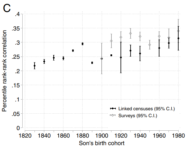
But this is not the end. Their conclusion relies much on the trends in the 1910-1940 cohorts. Yet Figure 3C from Song et al. (2020), who analyzed the IPUMS as well, indicates no difference between 1910 and 1940 and only a marginal decline in mobility thereafter (if we ignore the large confidence intervals, that is…). These authors maintain however that, between 1820 and 1980 cohorts, there was a small long-term decline in mobility. They excluded farm-origin sons because the industrialization process during the 19th century caused a sharp decline in the agricultural population which then caused sons of farmers to experience more upward mobility by migrating from farms to booming cities. This anomaly had to be corrected, and the graph below shows the result.
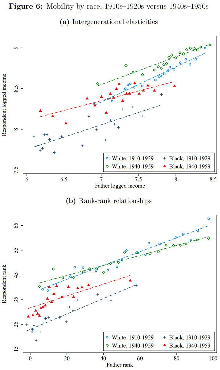
Ward (2021) also looked at historical census data and “confirmed” Jacome’s findings. Ward said that past research on the early 20th century and before are likely erroneous due to measurement error biasing mobility upward and the omission of Black families before “emancipation”. Occupational miscoding was substantial with the 1880 St. Louis Census. Racial disparities were wider in the past. Correcting for these artefacts, measurement error dealt with by using Instrumental Variables (IV) regression, he estimated father-son correlation in Figure 1 to be oscillating between 0.84 and 0.61 from 1840 to 1910 birth cohorts versus 0.44 and 0.37 from 1960 to 1980 birth cohorts. Figure 7 suggests that emancipation didn’t help Blacks to close the relative mobility gap since the inclusion of Blacks didn’t have differential impacts on the estimates across 1840 and 1910 cohorts. Because income data was unavailable long ago, occupation was used and based on literacy/education at the individual level adjusted for race and region’s level, in order to capture possible inequalities within occupation across race and region. As for the 1960-1980 cohorts, Ward uses the occupation variable of the PSID only, because unlike other surveys it contains multiple observations of occupation over the years, allowing averaging to reduce measurement error in the same way as the historical data.
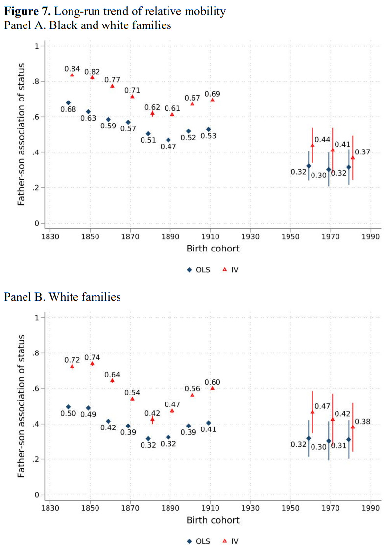
Ward concludes that research analyzing the mobility trend after the 1960 cohort reveals a flat, stable rate of relative mobility and would seem to contradict Great Gatsby (Chetty et al., 2014a; among many others). But he also notes that the long run evidence of the inequality-(im)mobility relationship over time is consistent with the Great Gatsby curve because 1) inequalities in the 19th and early 20th century have been estimated to be higher than today and because 2) this relationship has been weakened over time due to institutional changes that improved outcomes of poor families. The first point ignores that between 1830 and 1880 cohorts, the correlation declined gradually from 0.72 to 0.42 but then increased gradually to 0.60 until 1910 when looking at White families only, as it makes little sense to include anomalies such as enslaved people to make such a comparison. Dropping the sons of farmers as another anomaly doesn’t alter the estimates at all, but then Ward failed to provide an explanation for these extraordinary shifts in mobility. The second point requires investigation. Regarding trends, Davis & Mazumder (2022) informed us that mobility has decreased since 1980 but remained stable during the 2000s, consistent with the timing in Chetty et al. (2014a) later birth cohorts. But inequality was still rising, although at a slower pace. As for social welfare, Chetty et al. (2014b) reported a correlation of 0.32 between absolute upward mobility and local tax rates across U.S. states but also a correlation of -0.578 between inequality and mobility across U.S. states, both of which support Ward’s suspicions assuming no confoundings.
With respect to the racial gap though, Collins & Wanamaker (2022) confirmed my suspicions about Ward’s intriguing Figure 7. Instead of using single or even averaged year income which might be a noisy measure of permanent income (therefore overestimating mobility), they opt for occupation-based “income” measures of fathers’ status which are robust to temporary shocks (e.g., unemployment). They also use rank regression instead of log-linear regression as a further check against measurement error. Using the census data completed with OCG and NLSY79, the analysis of cohorts from 1900 to 1990 shows that the Black mobility stayed more or less constant over time, implying that the Civil Rights didn’t cause a visible shift. Either there were confounding factors or such impactful policies had simply no effect.
Of particular importance, the authors estimated “counterfactuals” for Blacks, which are estimates of the density of Black sons’ status conditional on the density of White sons’ status while retaining the distribution of Black fathers’ status. Put it simply, this model treats Black sons as if they had the mobility/transition of White sons. Because Figure 5 shows that Black men achieve occupation close to White men in all cohorts under counterfactual transitions, they believe mobility gap is the main reason for the persistence of earnings/occupation gaps.
If that is true, then the answer as to which factor causes mobility is urgently needed. Bloome et al. (2018) provided an interesting argument. They observe that parent income has become less predictive of adult income within education levels across NLSY79 and NLSY97 cohorts. The increasing educational inequality along with increasing educational returns would have decreased mobility while educational expansion along with the decline of parent-children income correlation would have increased mobility. Why educational expansion likely increases (upward) mobility for lower-class families is because the parent-children income correlation among college graduates is much weaker. Overall, these offsetting forces may have obscured the relationship between inequality and mobility. By how much is unclear though, especially after considering the finding that income mobility reduces substantially at the upper extreme of educational levels, that is, among PhD holders (Torche, 2011, 2018), combined with the finding that income inequality is mostly driven by the top 1% income (Piketty & Saez, 2003). Worse is that Zhou (2019) discovered that the seemingly high mobility of these college graduates as opposed to non-graduates was the product of selection process. These two groups had in fact similar mobility. Purging selection was done through a novel technique by Zhou, called residual balancing: “This method creates a set of weights such that in the reweighted sample, observed pre-college characteristics are no longer associated with college graduation at each level of parental income.” In the end, it doesn’t seem that educational expansion really promotes equality of chances.
Meanwhile the argument that education premium has increased didn’t lose force. To illustrate, Davis & Mazumder (2022) showed that the decline in mobility in the U.S. during the 1980-1990s can be easily accounted for by the increasing returns to education and the sharp increase in correlation between income and marriage.
All of these offsetting forces make analysis exceedingly complex. Hence, a question worth asking is how one can simulate the mobility gain of Blacks net of adverse external factors. Derenoncourt (2022) provided perhaps one such answer. She considers the second wave of the Black Migration (i.e., between 1940 and 1970) as one crucial natural experiment. As Blacks tried to settle in northern cities in number, the cultural and political response apparently neutralized the potential gain from moving up in destination locations. The dramatic rise in criminality, race riots and residential segregation caused a sharp increase in government expenditures on police, crowding out investment in education. The end result was the rise of incarceration for Black men and the flight of many Whites away from these urban neighborhoods. To disentangle these forces, the analysis involved a counterfactual model in which the upward mobility of Blacks moving North is estimated conditional that the Great Migration did not happen. The estimated gap was 9.1 percentiles. A disappointing result considering the above reports of the usual mobility gap.
Chetty et al. (2014b) noticed there is a large variation in mobility across U.S. states. When they regress the absolute mobility on both the areas’ fraction of single-parent families and share of black residents, the latter is no longer correlated with mobility. Single parent, rather than race, accounts for absolute upward mobility among Blacks.
Chetty et al. (2020) examined the most plausible factors of the BW mobility gap using data from the Census 2000 and 2010 and data from federal income tax returns between 1989 and 2015. Blacks have relative mobility comparable to Whites but lower absolute mobility. Even when moving across the parental income distribution, a similar gap is observed. Blacks with parental income at the 25th percentile earn 12.6 less while at the top 1% Blacks still earn 12.4 less than Whites.
The authors believed the situation of Black men is concerning because Black women won’t be able to close the gap if they are less likely to be married and have lower levels of household income because Black men earn much less than White men. Therefore, they evaluate one by one the other most likely factors of the BW gap when controlling for parent income.
The first control is marital status. They evaluated its effect by looking at individual incomes (i.e., excluding spousal income) and found that the gap is about 5 percentiles as opposed to 13 in household income. Strong effect? No, because a gloomy picture emerges after gender split. Black men earn 11 percentiles less than White men while Black women earn 1 percentile more than White women. There is no gap in wage rates or hours of work or even employment rates between Black and White women, and marital status only reduces the gap by 0.7 percentile or less among men.
One other important control is incarceration. Yet among Black men born to parents in the top 1%, their earnings ranks are still 10.2 percentiles below White men. Incarceration also fails to explain outcome disparities observed at younger age such as high school dropout rates.
Then comes parental wealth proxied by mortgage payments, home ownership, home value, number of vehicles. For males, the gap reduced from 9.1 to 8.0 percentiles after correcting for measurement errors of these proxies.
Their next control is neighborhoods. Upward mobility for both Blacks and Whites vary substantially across areas. There are substantial BW differences within virtually all commuting zones. When Blacks and Whites grow up in families with comparable incomes in the same neighborhood, implying they attend the same schools as well, the mobility gap reduces by only 30%, from 10 to 7 percentiles. Even more disconcerting is that they found that the gap increases by 2.5 percentiles when moving from the highest poverty to the lowest poverty neighborhoods. And when the authors examine only men, the same pattern emerges. The gap increases in high quality neighborhoods. Several factors, still, moderate the gap. Comparing the lowest and highest levels of father presence reduces the gap from 9.3 to 6.1 percentiles.
The final control accounts for racial bias, either measured by the Implicit Association Test or the Racial Animus Index. Counties with a one SD higher level of bias against Blacks among Whites would be associated with 0.8 percentiles lower income ranks for either Black men or Black women.
While these controls exert little to modest effect, they probably overlap by a large extent. And all of these are mediated by IQ anyway as research proved it. Yet at some point Chetty et al. (2020, p. 751) tried to discard the “IQ thesis” on the basis that there is no gender gap in IQ while a large gender gap exists in mobility. This must be a joke. First, IQ-income correlation is very far from 1. Second, both variables certainly aren’t caused by the same external effects. Third, confoundings or offsetting forces can have different impacts on income across gender. Fourth, parent income hardly transfers to the children (as seen with the low reported r everywhere) which is completely the opposite for IQ. Likewise, I would look like a fool for discarding IQ as a factor of income just because the St. deviation of IQ has modest correlation with Gini across countries or that Blacks exceed Whites in income at high levels of IQ. If Chetty et al. didn’t downplay IQ, they would likely reach a conclusion similar to Mazumder (2014).
Indeed, Mazumder (2014) analyzed the BW mobility gap among men as measured by transition probabilities using the NLSY79 as well as the SIPP-SSA. Income was averaged across years and between ages 33-48. What is interesting here is that the SIPP-SSA has administrative earnings records. Such an index is more reliable than self-reported income as it was sometimes argued that very low income people may over-report and very high income people may under-report. But Figures 1-2 show very small differences between the data. Of more importance is that NLSY allows one to control for AFQT, and the result is shown below. Quite impressive.
But as always, nothing looks easy. Davis & Mazumder (2018) observed that the variation in mobility across races is much larger than across U.S. regions. Accounting for AFQT in the NLSY79 drastically reduces the BW gap uniformly across regions, yet the variation in mobility across regions remains non-trivial. It does not imply that regional differences have anything to do with racial differences but a question worth asking is whether the causes of regional differences can exert a stronger and lasting effect on Blacks. If public policy is the main cause, then the above findings suggest there is little hope.
On the other hand, it is fairly possible that such high variation across regions was merely an illusion. Mogstad et al. (2020) argued that Chetty’s (2014b) measure, also used by Davis & Mazumder (2018), of locational upward mobility is not precise. Chetty’s measure was: The expected income rank of children who grew up in a given area with parents at the 25th percentile of the income distribution of parental income. Because they are comparing areas’ estimates, not the classical (also called marginal) confidence interval (CI) but rather the simultaneous CI must be computed. The problem is that the simultaneous CI is the product of all of the areas’ CI that the simultaneous CI is supposed to cover at 95%. And once the 95% simultaneous CIs for the ranks of all areas are calculated and displayed (Figure 6A-6B), one sees clearly that the overlap is so substantial that one cannot draw strong inferences about which area is more mobile.
Where are we going from here?
Policy makers strongly and wrongly believe equalizing chances would play a huge role in reducing income/education differences. When it comes to the BW gap, IQ solely accounts for almost the entirety of the mobility gap and a smaller but still substantial variation of the wage gap. The Civil Rights did not improve Blacks’ outcomes and the Black Migration even worsened their outcomes. Many methods were tried to reduce the gap, and their failures never stopped the exploration of unknown methods. It is true that the failure to find a tiger in the forest does not mean there is no tiger (although the likelihood decreases as you search further). The consequence is that over time, people are relying more and more on the government, for just about everything. And this has a cost most don’t (or refuse to) see. Historical records abound of examples about regulation causing moral hazard behaviour, ultimately requiring further intervention. A beginning of a vicious cycle. The banking system being the best instance of such misfortune.
One wonders whether relative mobility is truly more important than absolute mobility or if relative poverty matters more than absolute poverty. Economic freedom promotes growth, productive investment, which in theory improves even more absolute mobility and wealth as children are much better off than their parents “ceteris paribus”. Public policies are often accompanied with unintended consequences hurting the poor families to some extent. This is something you don’t often hear from mainstream economists. Empirically we have some evidence that regulation lowers innovation (Aghion et al., 2021) and that innovation with two-year lag is associated strongly with top income inequality (but not broad measures) and moderately with absolute upward mobility across U.S. states (Aghion et al., 2019). Various indices of economic freedom also correlate with absolute mobility across nations (Callais & Geloso, 2021). A finding at odds with people championing the conclusion of the Great Gatsby. Many reports confirmed that the productivity of human capital depends on the quality of institutions (a proxy for economic freedom) such that human capital leads to increases in output (Ihlenfeld et al., 2022). Generally, state-level economic freedom increases real income across U.S. states (Hall et al., 2019) and also reduces the adverse impact of economic crisis such as the Great Recession (Callais & Pavlik, 2022). And as astounding this appears to be, economic freedom also reduces Black-White health disparities in the U.S. after accounting for various demographic and socio-economic variables (Hall et al., 2015). One wonders whether fighting inequalities doesn’t lead one to miss a much bigger picture.
References
- Bloome, D., Dyer, S., & Zhou, X. (2018). Educational inequality, educational expansion, and intergenerational income persistence in the United States. American Sociological Review, 83(6), 1215-1253.
- Cheng, S., Tamborini, C. R., Kim, C., & Sakamoto, A. (2019). Educational variations in cohort trends in the black-white earnings gap among men: Evidence from administrative earnings data. Demography, 56(6), 2253-2277.
- Chetty, R., Hendren, N., Kline, P., Saez, E., & Turner, N. (2014a). Is the United States still a land of opportunity? Recent trends in intergenerational mobility. American Economic Review, 104(5), 141-47.
- Chetty, R., Hendren, N., Kline, P., & Saez, E. (2014b). Where is the land of opportunity? The geography of intergenerational mobility in the United States. The Quarterly Journal of Economics, 129(4), 1553-1623.
- Chetty, R., Hendren, N., Jones, M. R., & Porter, S. R. (2020). Race and economic opportunity in the United States: An intergenerational perspective. The Quarterly Journal of Economics, 135(2), 711-783.
- Collins, W. J., & Wanamaker, M. H. (2022). African American intergenerational economic mobility since 1880. American Economic Journal: Applied Economics, 14(3), 84-117.
- Daly, M. C., Hobijn, B., & Pedtke, J. H. (2017). Disappointing facts about the black-white wage gap. FRBSF Economic Letter, 26, 1-5.
- Daly, M. C., Hobijn, B., & Pedtke, J. H. (2020). Labor market dynamics and black–white earnings gaps. Economics Letters, 186, 108807.
- Davis, J., & Mazumder, B. (2018). Racial and ethnic differences in the geography of intergenerational mobility. Available at SSRN 3138979.
- Davis, J., & Mazumder, B. (2022). The decline in intergenerational mobility after 1980.
- Derenoncourt, E. (2022). Can you move to opportunity? Evidence from the Great Migration. American Economic Review, 112(2), 369-408.
- Jácome, E., Kuziemko, I., & Naidu, S. (2021). Mobility for all: Representative intergenerational mobility estimates over the 20th century (No. w29289). National Bureau of Economic Research.
- Mazumder, B. (2014). Black–white differences in intergenerational economic mobility in the United States. Economic Perspectives, 38(1).
- Mogstad, M., Romano, J. P., Shaikh, A., & Wilhelm, D. (2020). Inference for ranks with applications to mobility across neighborhoods and academic achievement across countries (No. w26883). National Bureau of Economic Research.
- Muller, S. M. (2008). Begging the question: permanent income and social mobility (No. 75). Economic Research Southern Africa.
- Muller, S. M. (2010). Another problem in the estimation of intergenerational income mobility. Economics Letters, 108(3), 291-295.
- Ren, C. (2022a). A Dynamic Framework for Earnings Inequality between Black and White Men. Social Forces, 100(4), 1449-1478.
- Ren, C. (2022b). Cohort, signaling, and early-career dynamics: The hidden significance of class in black-white earnings inequality. Social Science Research, 102710.
- Song, X., Massey, C. G., Rolf, K. A., Ferrie, J. P., Rothbaum, J. L., & Xie, Y. (2020). Long-term decline in intergenerational mobility in the United States since the 1850s. Proceedings of the National Academy of Sciences, 117(1), 251-258.
- Thompson, O. (2021). Human Capital and Black-White Earnings Gaps, 1966-2017 (No. w28586). National Bureau of Economic Research.
- Torche, F. (2011). Is a college degree still the great equalizer? Intergenerational mobility across levels of schooling in the United States. American journal of sociology, 117(3), 763-807.
- Torche, F. (2018). Intergenerational mobility at the top of the educational distribution. Sociology of Education, 91(4), 266-289.
- Ward, Z. (2021). Intergenerational mobility in American history: Accounting for race and measurement error (No. w29256). National Bureau of Economic Research.
- Zhou, X. (2019). Equalization or selection? Reassessing the “meritocratic power” of a college degree in intergenerational income mobility. American Sociological Review, 84(3), 459-485.
Discover more from Human Varieties
Subscribe to get the latest posts sent to your email.

I think it’s worth noting that the stenze 2007 meta-analysis didn’t find appreciable growth over time to the returns of IQ in terms of either of the three outcome variables.
If you were thinking of his Table 2, yes, there is no trend for either education, occupation and income. I’m not saying I don’t trust Strenze, because the article is really well written and he proved he knows what he is talking about and seemed to have looked at those studies somewhat deeper. But I’m still concerned about income which didn’t improve its correlation with IQ after correction for attenuation, unlike education and occupation, and given the fact that income varies so greatly over one’s lifetime, and its effect depends greatly on the time it has been measured. I don’t know how much I can trust these numbers, as I still have the feeling these figures could be (differentially over periods?) biased downward. I can read those studies, provided I have time and motivation.
Regarding higher educational attainment in black students after controlling for test scores, this is something I noticed ~15 years ago when I realized that black college graduation rates are much higher than would be expected based on test scores, and I’ve seen it acknowledged in a few papers here and there.
This makes more sense when you consider that the black-white test score gap is only modestly reduced by controlling for parental SES. A corollary of this is that black students tend to come from higher-SES backgrounds than white students with the same test scores.