The SAT is the most popular standardized test used for college admissions in the United States. In principle, SAT scores offer a good way to gauge racial and ethnic differences in cognitive ability. This is because, psychometrically, the SAT is just another IQ test–that is, it is a set of items the responses to which can be objectively marked as correct or incorrect.[Note 1] Unsurprisingly, SAT scores correlate strongly with scores from other IQ tests (Frey & Detterman, 2004). It is also advantageous that SAT-takers are generally motivated to get good scores, and that large numbers of young people from all backgrounds take the test each year, enabling precise estimation of population means.
However, the SAT has at least two major limitations when used for group comparisons. Firstly, it is a high-stakes college entrance test, which means that it is a target for intense test preparation activities in ways that conventional IQ tests are not, potentially jeopardizing its validity as a measure of cognitive ability. Secondly, taking the SAT is voluntary, which means that the participant sample is not representative but rather consists of people who tend to be smarter and more motivated than the average.
This post will attempt to address these shortcomings. I will investigate whether racial and ethnic gaps in the SAT are best understood as cognitive ability gaps, or if other factors make a significant contribution, too. An important method here is to compare the SAT to other tests that are not subject to extraneous influences such as test prepping. Another goal of the post is to come up with estimates of racial/ethnic gaps in the test that are minimally affected by selection bias. This can be done with data from states where entire high school graduate cohorts take the SAT. Other topics that will receive some attention in the post include ceiling effects, predictive validity, and measurement invariance.
Because racial/ethnic gaps in the SAT have changed over time, an essential part of the analysis is understanding these temporal trends. In particular, Asian-Americans have performed extraordinarily well in the test in recent years. Getting a better handle on that phenomenon was a major motivation for the post. Comparisons of trends in the national and state-level results turned out to be informative with respect to this question.
The post is multipronged and somewhat sprawling. This is because the (publicly available) SAT data do not yield straightforward answers to many important questions about racial and ethnic differences. The only way to get some clarity on these issues is to examine them from multiple angles, none of which alone supplies definitive answers, but which together, hopefully, paint a reasonably clear picture. I have relegated many technical details of the statistical methods used, as well as many ancillary analyses, to footnotes so as make the main text less heavy-going. The data and R code needed to reproduce all the calculations, tables, and graphs in this post are included at the end of each chapter, or, in the case of some ancillary analyses, in the footnotes.
[toc]
1. Racial and ethnic gaps over time
I will start by overviewing the evolution of racial/ethnic gaps in the SAT in the last few decades. I will first analyze national data, as opposed to state-level data. While the national data have known weaknesses, especially self-selection bias, they nevertheless offer a useful starting point. The racial/ethnic gaps that the admissions officers of selective colleges encounter reflect the national data, and, generally, racial/ethnic gaps in self-selected samples are at least moderately correlated with gaps in representative samples. I will later compare the national results to results from selected states.
The SAT has been revised several times in recent decades. Before 2006, the test had two sections, Verbal and Math, both scored on a scale of 200 to 800, so that the minimum total, or composite, score was 400, while the maximum total score was 1600. In 2006, the Verbal section was replaced with two new sections called Critical Reading and Writing, and each section was scored on a scale of 200 to 800, so that possible total scores ranged from 600 to 2400. In 2017, the Critical Reading section was replaced with a section called Evidence-based Reading and Writing (ERW), the Writing section was made optional, and the old total or composite score scale was restored (i.e., ERW + Math equals 400 to 1600). Until recently, a range of more narrowly focused tests called SAT Subject Tests, or SAT II tests, were also administered. I will ignore them in this post.
In the SAT, raw scores, which are computed as the number of correct responses minus possible penalties for incorrect responses (see below), are converted into SAT scale scores so that the latter rise by 10 point increments, e.g., 500, 510, 520, etc. The composite score mean (verbal + math) of the entire national cohort has historically been around 1000. The SDs of each SAT section have traditionally been roughly 100, while the total score SDs have been a bit more than 200 (two sections) or 300 (three sections).
The background information provided by SAT takers includes self-identified race or ethnicity. The racial/ethnic groups traditionally recognized are white, black, Hispanic, Asian/Pacific Islander, Native American, and “Other”. Some students skip this question (“No Response”). This categorization was revamped in 2016 when Asians and Pacific Islanders were split into two separate groups, and the category “Two or More Races” was added. There also used to be three Hispanic/Latino categories–Mexican, Puerto Rican, and other Hispanic/Latino–but since 2016, all Hispanics/Latinos have been pooled together (I will be using the pooled category throughout). The “Other” race/ethnicity option was discontinued beginning in 2017.
SAT means disaggregated by race/ethnicity are available from reports published by the College Board, which owns the test. National and state-level reports since 2016 can be downloaded here. Earlier reports are somewhat harder to locate, but many can be found by doing Google site searches on https://secure-media.collegeboard.org. The following list has links to the College Board’s reports on national SAT score distributions from 2002 through 2022. Here and throughout this post, the years associated with SAT data refer to the high school graduation year of the test-takers in each cohort.
- 2002
- 2003
- 2004
- 2005
- 2006
- 2007
- 2008
- 2009
- 2010
- 2011
- 2012
- 2013
- 2014
- 2015
- 2016
- 2017
- 2018
- 2019
- 2020
- 2021
- 2022
I supplemented the College Board data with some from The Digest of Education Statistics. In particular, The Digest data include racial/ethnic SAT means from selected years predating 2002, allowing me to extend the time series further back.[Note 2]
Figure 1.1 shows the evolution of the racial/ethnic mean scores in the SAT at the national level from 1987 through 2022. The scores used are composite or total scores formed by summing the math sections, and the (variously labeled) verbal sections. From 2006 to 2016, the writing sections are included in the sums, too. From 2017 on, the total mean scores can be readily found in the College Board’s reports, but for earlier years I calculated the total scores as simple, unweighted sums of the section mean scores.[Note 3]
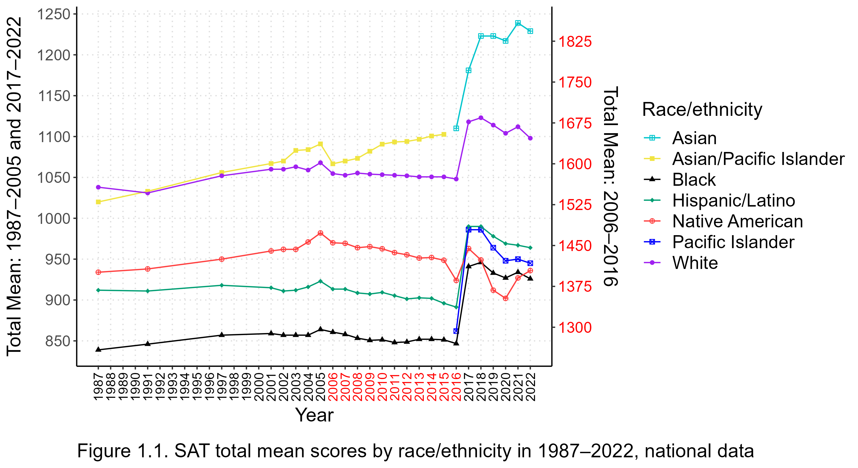
Because the range of feasible SAT scores has changed over time, as explained above, the y-axis on the left-hand side of Figure 1.1 applies to years before 2006 and after 2016, while the y-axis on the right-hand side applies to the years 2006–2016 (marked in red on the x-axis). The mean scores from 2006 through 2016 have been rescaled so that their units have a visual size 

From Figure 1.1, it is clear that 2017 was a watershed year for the SAT: the mean scores of most groups shot up, and the size of many racial and ethnic gaps changed as well. It was also the year of the latest major revision of the test.[Note 4]. Mean scores (on the 400 to 1600 scale) and group differences had been relatively stable for thirty or more years before 2017, so it is tempting to draw the conclusion that changes in the test itself caused the upheaval in the results. However, such a conclusion would be premature because the introduction of the revised SAT coincided with large increases in test participation. Figure 1.2 depicts changes in the numbers of SAT-takers overall and by race/ethnicity since 2002.
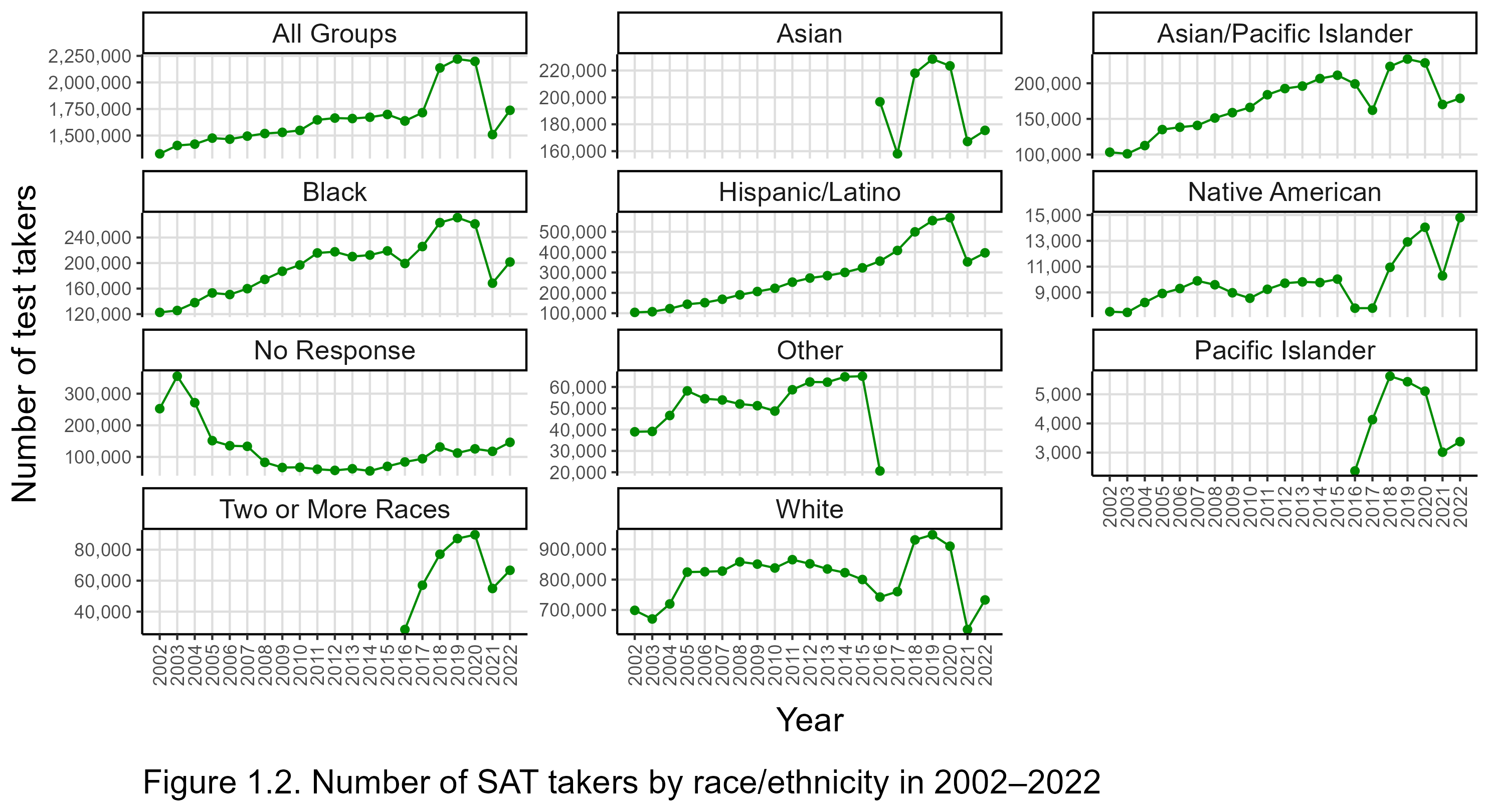
Overall, there were around 1.5 to 1.7 million annual test-takers in 2005–2017, then 2.1 million in 2018, and a record 2.2 million in 2019 and 2020. This turnaround was apparently caused by the decision of a number of states and school districts to pick up the tab for high-schoolers to take the test each year. Notably, 2017 was a transitional year because of the revision, causing some unusual shifts in participation, e.g., a large temporary dip in the Asian numbers.[Note 5] For this reason, data from 2018 and later are more informative about the redesigned SAT’s impact.
From Figure 1.2, it can also be seen that participation declined sharply after the double whammy of the coronavirus pandemic and the “racial reckoning” hit in 2020. The pandemic caused the College Board to cancel test administrations, and many colleges stopped asking for test scores for the duration. Meanwhile, the Black Lives Matter movement went into high gear, and among its demands was that test scores be banned in college admissions so as to give a leg up to low-scoring groups like blacks and Hispanics.
I will return to the question of what effect these changes in the composition of the test-taking cohorts had, but I will first look at the test score trends in more detail to get a better descriptive sense of what happened. One thing to note upfront is that the shifts in group differences that happened in 2017 were generally retained when there was a large drop in the number of test-takers after 2020.
With the exception of Native Americans, the mean scores of all groups considered here increased permanently after the 2017 revision, stabilizing at values substantially above their long-term trends on the 400 to 1600 scale. Considering that this happened while test participation was becoming less selective, SAT scales before and after 2017 are incommensurate, and should not be used for direct ability comparisons.
Again with the exception of Native Americans, from 1987 through 2022, all groups achieved their highest mean scores after the introduction of the redesigned SAT in 2017. On average, the means over the 2017–2022 period differ from the means over the 2002–2016 period on the 400 to 1600 scale in the following way:
| Group | Old mean | New mean | Difference: new–old |
|---|---|---|---|
| Asian/Pacific Islander | 1089 | 1214 | 125 |
Changes in test content are a potential explanation for why people are scoring higher in the revised SAT. David Coleman, the president of the College Board since 2012, is one of the architects of the Common Core educational standards that describe what students should know and be able to do in each grade level. The Common Core has had a major influence on states’ K-12 curriculum standards. A central motivation for the 2017 SAT revision was to tie the test to the Common Core standards. One goal seems to have been to emphasize skills and knowledge with “real-world applications”. For example, the Technical Manual of the test asserts (p. 15) that the knowledge of “obscure” words is no longer rewarded in the SAT. Historically, the SAT has not been designed to be aligned with school curricula, so the revised version appears to break with this tradition. Moreover, while the College Board had previously been dismissive of test prep, since 2015 it has partnered with Khan Academy to provide free online SAT prep resources.
Another potential explanation for the boost in scores since 2017 is changes in the way the test is scored. The SAT used to penalize incorrect responses, with 
The SAT total or composite score mean for all test-takers on the 400 to 1600 scale has historically been close to 1000, varying between 989 and 1028 over the period of 1987 to 2016 (although see [Note 2]). Accordingly, the College Board wanted both sections of the revised SAT to have means of “500 for a college-bound group weighted to reflect the old SAT cohorts” (Technical Manual, p. 76), and thus a total score mean of 1000. However, after the new test was first administered in 2017, the total score mean of all test-takers has always been substantially higher than that, ranging from 1050 to 1068. This happened despite the fact that the number of SAT-takers increased by more than 30 percent in the first years after the redesigned SAT was adopted, almost certainly causing the test-taking cohorts to be less cognitively selected than before. Students found the new test easier than the College Board had intended. In this respect, the 2017 redesign compares unfavorably to the 2006 redesign which, as can be seen from Figure 1.1, more or less preserved the established meaning of the SAT scale points even when a new section, Writing, was added to the test. Then again, it is possible, as suggested in this article, that the inflation of scores in the new SAT was intentional, designed to make the test more attractive to test-takers than its sole competitor, the ACT.[Note 6] However, the test score shifts associated with the redesign differ considerably between groups, so they cannot be solely a matter of moving the midpoints of the scales.
The most conspicuous change in ethnic and racial gaps since 2017 is the skyrocketing of Asian American test performance. Asian Americans had been gradually pulling away from others at least since 2000, but after 2017 they have completely outstripped the competition. The Asian-white gap, for example, is now well over 100 points, whereas it was less than 50 points relatively recently.[Note 7]
Among low-performing groups, the 2017 revision caused a substantial narrowing of differences in the sense that blacks, Hispanics, Native Americans, and Pacific Islanders now have mean scores very close to each other. The plummeting of the test scores of Native Americans since 2017 is noteworthy. They used to consistently outperform Hispanics and blacks, but now they are at the bottom of the rankings with blacks. The reason for this shift is unknown.
Another way to look at racial/ethnic differences is to standardize them so that the gaps show how many SDs higher one group scored than another. This sidesteps the problems caused by changes in the SAT scales over time while also enabling comparisons with other tests and variables. Additionally, standardized gaps adjust for unequal SDs that affect gaps expressed in unstandardized scale units.
Throughout this post, I will use Cohen’s d to compute standardized gaps. It is computed by dividing the unstandardized score difference by an SD pooled across the groups being compared:

where d is the standardized gap, while 


where 


The means of composite tests can be calculated by summing the section means, but composite SDs, which are needed so that d gaps can be calculated, depend on both the SDs of the sections and the correlations between them. This information is not readily available in the College Board’s reports, and it must be estimated in various ways. The statistical procedures used to arrive at d estimates are explained in [Note 8].
Figure 1.3 shows standardized racial/ethnic gaps in SAT total scores from 2002 through 2022 (gaps for earlier years are not available because of data limitations). The white mean is always at the zero point on the y-axis, and gaps are expressed as differences from whites. Positive gaps indicate that the other group scored higher than whites, while negative gaps indicate that whites scored higher.
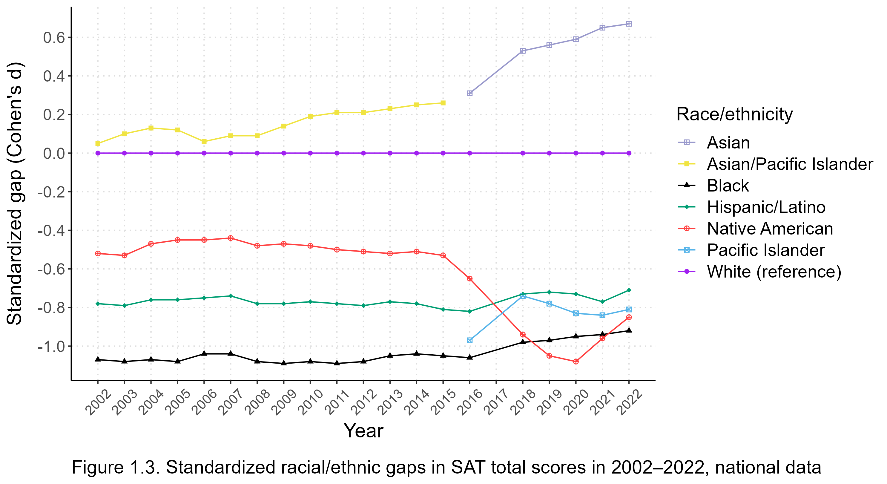
Figure 1.3 has no data for 2017 because the College Board has not published information on the within-group variability of the SAT for that year, making it impossible to properly calculate standardized gaps. However, the unstandardized data in Figure 1.1 confirm that 2017 was indeed a turning point for the SAT. In particular, Asians were only slightly ahead of whites in the immediately preceding years, with d values ranging from 0.20 to 0.30, until the revised SAT put them on a whole new growth trajectory so that by 2022 the Asian-white gap was a whopping d = 0.67. Moreover, the white-black and white-Hispanic gaps had long been stable at around d = 1.05 and d = 0.80, respectively, but after 2017 both gaps decreased somewhat. Meanwhile, Native American test scores cratered with the redesigned SAT.
One potential explanation for the changes in the gaps after 2017 is that the Writing section, which was a part of the SAT in 2006–2016, was made optional. This had the effect of giving mathematical ability more weight than before in the calculation of total scores. To explore this issue, I replotted the unstandardized and standardized total score gaps while omitting the Writing section for the period 2006–2016. In Figures 1.4 and 1.5, the dashed lines represent total scores computed from only verbal and math scores, while the solid lines represent total scores computed from all three sections (when available), matching the lines Figures 1.1 and 1.3. For clarity’s sake, all scores in Figure 1.4 are represented only on the 400 to 1600 scale, meaning that the three-section composites have been multiplied by
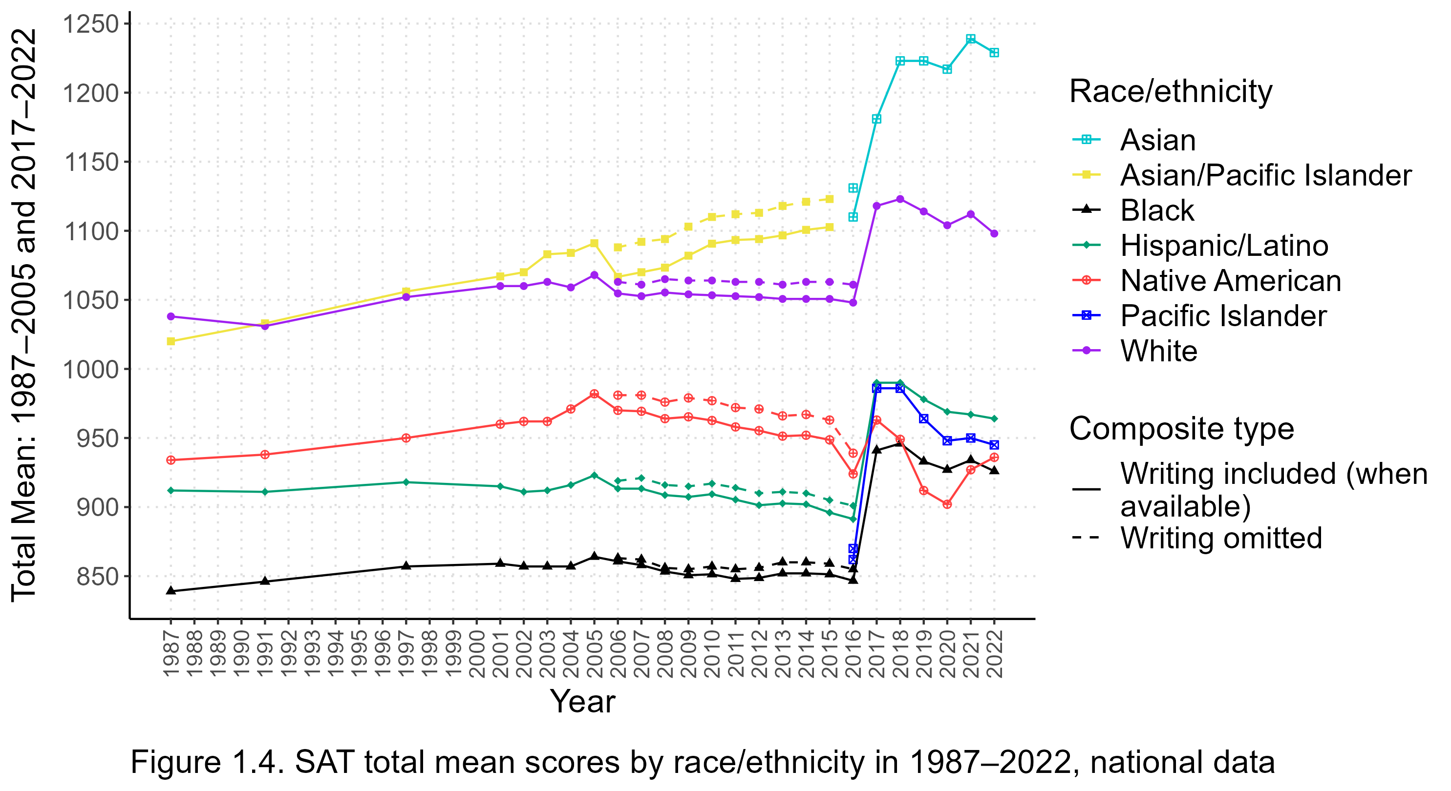

Figure 1.4 shows that when placed on the 400 to 1600 scale, the verbal + math composites are somewhat higher for all groups than the verbal + math + writing composites. More interesting is, however, Figure 1.5 which shows the standardized gaps. For blacks and Hispanics, the two- and three-part composites yield essentially identical gaps in relation to whites, while for Native Americans, omitting the Writing section narrows the gap to whites slightly. For Asians/Pacific Islanders, omitting the Writing section expands the gap to whites somewhat. This suggests that the removal of the mandatory Writing section from the SAT explains some of the supernormal gains that Asians experienced after 2017. However, in 2006–2015, the Asian/Pacific Islander-white gap in the two-part composite was only d = 0.05 higher, on average, than the gap in the three-part composite. This means that the removal of the Writing section can explain only a relatively small part of the Asian post-2017 gains which amount to d = 0.30 or so.
Next, let’s look at the evolution of the d gaps for the verbal section. Figure 1.6 depicts standardized verbal gaps from 2002 through 2022.

Asian Americans have historically performed relatively weaker in the verbal section of the SAT. In 2002, whites led Asians by about 0.25 SDs in it. In the following fifteen years, Asians gradually chipped away at the gap until they reached parity with whites around 2016. Then the redesigned test was released, and in a few years the verbal gap favored Asians by more than it had favored whites twenty years previously.
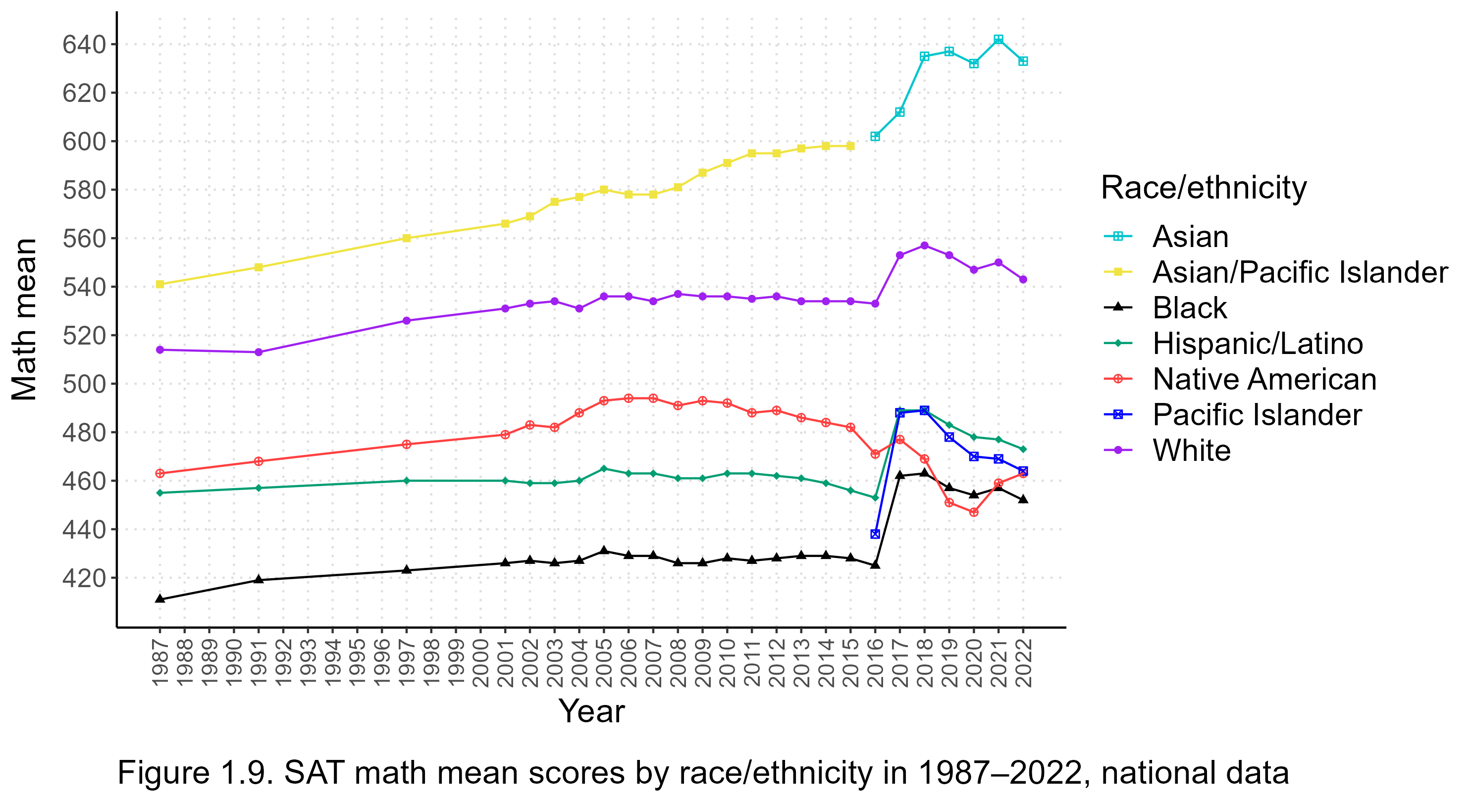
The math section has been a strong suit for Asian Americans for a long time, and continued to be so after the new test was released, as seen in Figure 1.7:

Even so, more of the greater-than-expected Asian gains in total scores seem to be due to the verbal section than the math section. Looking at the other groups, the new test seems to have stimulated black performance, in particular–after a long stagnation, they have modestly but unmistakably narrowed both math and verbal gaps. Native Americans fell behind in both sections.
I think the standardized gaps are more informative, but, for the sake of completeness, the following sections can be expanded for unstandardized verbal and math mean scores by race/ethnicity:
Figure 1.8. Unstandardized SAT verbal means
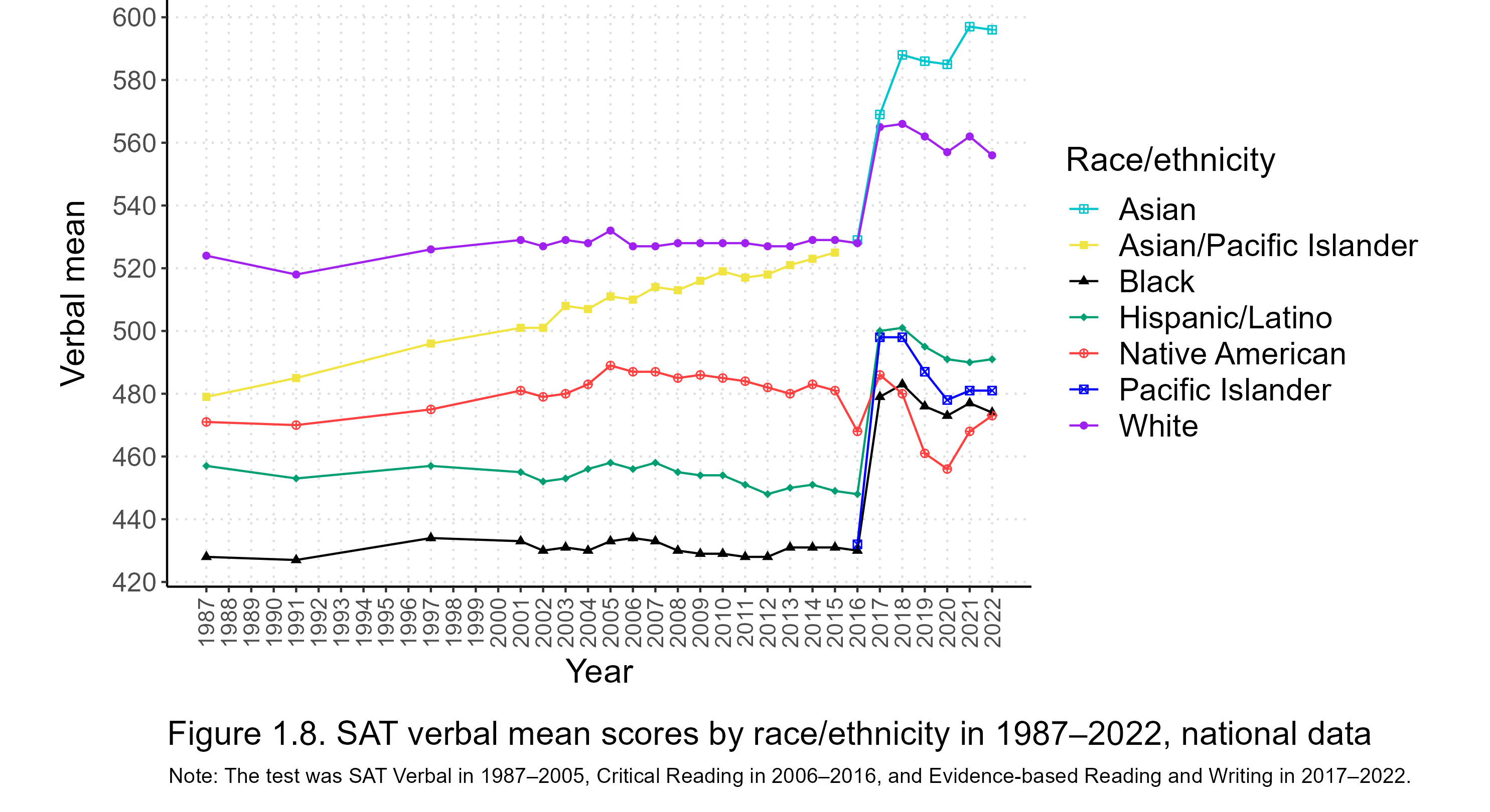
Figure 1.9. Unstandardized SAT math means
Looking at the pre-2017 gaps in Figures 1.3, 1.6, and 1.7, it is apparent that if the trends that existed then had continued, the gaps today would be rather different. The trend shifts can be quantified by regressing gaps on years in the pre-2017 data, and then using the resulting regression equations to predict how large the gaps would be post-2017 if the old trends had persisted. Figures 1.10 (total scores), 1.11 (verbal scores), and 1.12 (math scores) compare linear trends in standardized gaps in the two periods of interest, viz., 2002–2016 and 2018–2022 (gaps for 2017 are unavailable). The solid lines show the observed regressions, while the dashed lines show what the gaps would have been post-2017 if the pre-2017 trends had continued. The differences between the solid and dashed lines in the post-2017 period indicate the effect of the redesigned SAT on the gaps (which may be due to changes in the test itself, or due to changes in the composition of the test-taking cohorts). Gaps are shown in relation to whites for Asians/Pacific Islanders, blacks, Hispanics, and Native Americans. Asians and Pacific Islanders were grouped together throughout this analysis for continuity. For the period 2006–2016, the gaps used below are based on all three sections of the SAT, including Writing, so some of the post-2017 Asian total score gains can be explained by the removal of the Writing section, as discussed above.


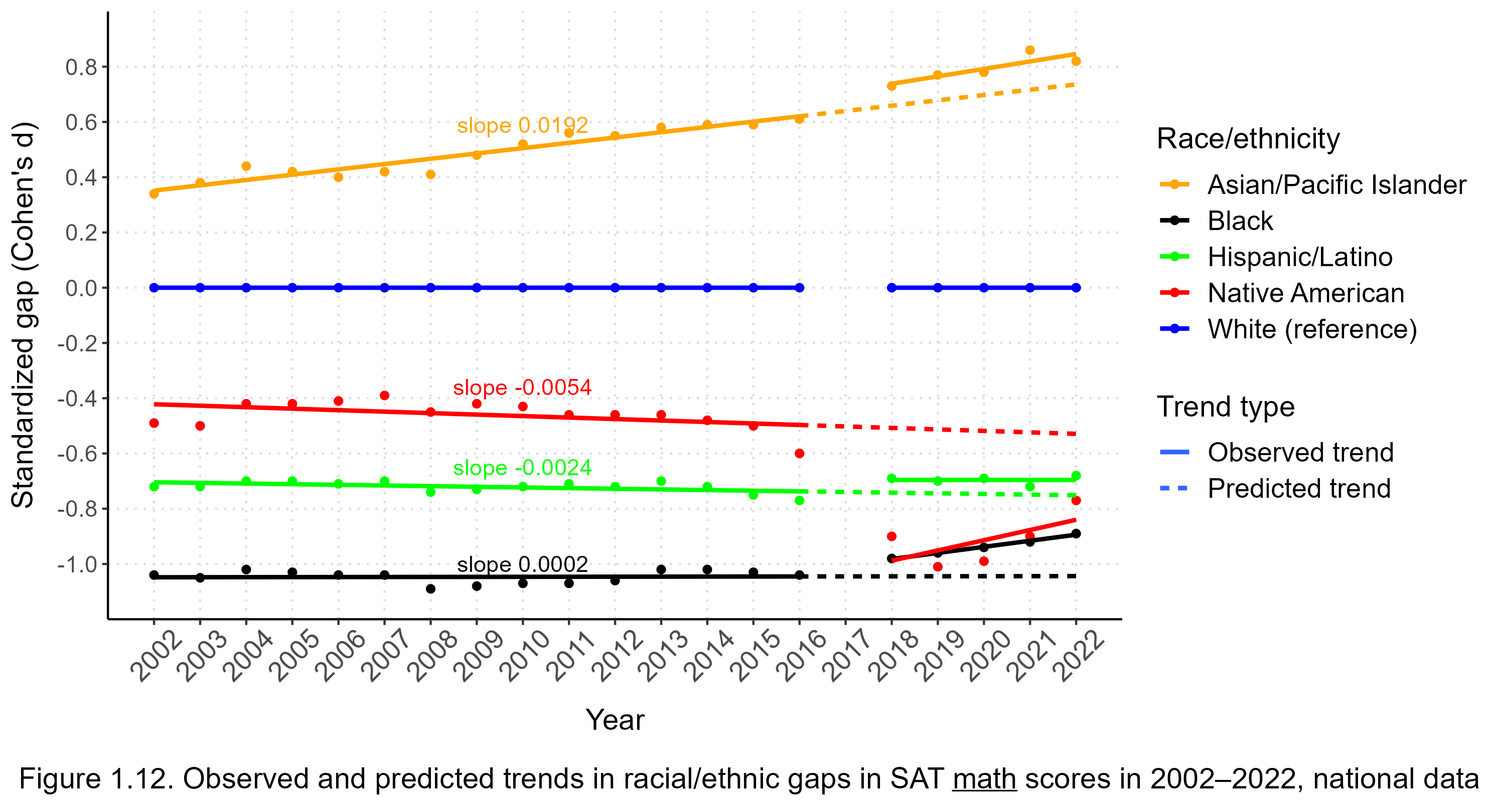
The slopes specified on the regression lines indicate how much each gap changed per year in the pre-2017 period, on average. Black and Hispanic trends were essentially stationary before 2017. Native American test scores were also quite stable in relation to whites before 2017, decreasing at a slow rate at most. Depending on the test, Asians were gaining on whites by d = 0.015 to d = 0.019 each year before 2017.
Despite the fact that the trajectories of racial/ethnic gaps are well-described by linear models in the pre-2017 period, none of the post-2017 gaps are well-predicted by the older data. Blacks and Hispanics gained modestly on whites after 2017, Asians gained considerably more, and Native Americans fell far more behind than ever before. While the post-2017 regression slopes (i.e., rates of change in gaps) are still rather uncertain (and therefore not shown numerically in the graph), so far it appears that Asians are now increasing their lead on whites faster than they did historically.
While Asians saw supernormal gains in math after 2017, their gains in the verbal section were greater, and verbal gains explain most of the Asian total score gains. This can be more precisely quantified by estimating what proportions of the differences between the observed and predicted total score gaps were due to verbal versus math scores. Between 2017 and 2022, an average of 71 percent of the greater-than-expected total score gains of Asians in relation to whites were due to the verbal section, while 29 percent were due to the math section. For the other groups, the contributions of verbal and math sections to the differences between observed and predicted gaps were, on average and respectively, somewhat more even: 41% and 59% for blacks, 60% and 40% for Hispanics, and 55% and 45% for Native Americans.[Note 9]
To summarize the basic trends in the national SAT data numerically, Table 1.2 compares the gaps predicted based on the pre-2017 data to the ones actually observed post-2017. Both the observed and predicted values are unweighted averages across the years 2018–2022.
| Verbal gap | Math gap | Total gap | |||||||
| Group | Observed | Predicted | Observed | Predicted | Observed | Predicted | |||
|---|---|---|---|---|---|---|---|---|---|
| Asian/Pacific Islander | 0.28 | 0.05 | 0.79 | 0.70 | 0.57 | 0.34 | |||
The data presented in this chapter give an overview of national racial and ethnic test score gaps in college-aspiring cohorts since 1987 (with more detail since 2002). The most important finding of this analysis is the way the 2017 redesign of the SAT disrupted long-established trends in the gaps. There were large and abrupt changes coinciding with the deployment of the redesign, especially in the performance of Asians and Native Americans in relation to others. The changes also persisted after participation declined steeply beginning with the high school graduating class of 2021.
Because of self-selection into the sample whose strength may vary by race/ethnicity and year, SAT gaps analyzed in this chapter do not correspond to ones that would be obtained by making random samples of high schoolers take the test. This bias may cause difficult-to-discern aggregation fallacies in the interpretation of trends in the racial/ethnic gaps. To attenuate this problem, in the next chapter I will look at SAT gaps in states where participation in the test remained constant over multiple years. This will enable better estimates of the true effect of the SAT redesign on the test performance of each group.
The following CSV tables contain all the SAT data and estimates discussed above. Note that the groups called Hispanic/Latino, All Groups, and (after 2015) Asian/Pacific Islander are composites of other included groups. The variables with Verbal in their name refer either to the Verbal, Critical Reading, or Evidence-based Reading and Writing section, depending on which label was used in a given year. Some statistics are missing (NA) for certain years because of lack of data. The tables also contain data for groups that were omitted from most of the analyses above to keep the graphs more readable (e.g., the “One or More Races”, “Other”, and “No Response” categories). Variables whose names start with Male or Female contain within-sex data, while variables with no such prefixes contain data pooled across the sexes (e.g., Female_Total_SD and Male_Total_SD versus Total_SD). The CSV tables throughout the post are presented for ease of reuse; they need not be loaded to run my R code.
SAT national data master table 1987–2022
Year,Group,Verbal_Mean,Math_Mean,Total_Mean,N,Verbal_SD,Math_SD,Total_SD,Writing_Mean,Writing_SD,Male_N,Male_Verbal_Mean,Male_Verbal_SD,Male_Math_Mean,Male_Math_SD,Female_N,Female_Verbal_Mean,Female_Verbal_SD,Female_Math_Mean,Female_Math_SD,Male_Total_Mean,Female_Total_Mean,Male_Total_SD,Female_Total_SD,Male_Writing_Mean,Male_Writing_SD,Female_Writing_Mean,Female_Writing_SD
1987,All Groups,507,501,1008,NA,NA,NA,NA,NA,NA,NA,NA,NA,NA,NA,NA,NA,NA,NA,NA,NA,NA,NA,NA,NA,NA,NA,NA
1987,Asian/Pacific Islander,479,541,1020,NA,NA,NA,NA,NA,NA,NA,NA,NA,NA,NA,NA,NA,NA,NA,NA,NA,NA,NA,NA,NA,NA,NA,NA
1987,Black,428,411,839,NA,NA,NA,NA,NA,NA,NA,NA,NA,NA,NA,NA,NA,NA,NA,NA,NA,NA,NA,NA,NA,NA,NA,NA
1987,Hispanic/Latino,457,455,912,NA,NA,NA,NA,NA,NA,NA,NA,NA,NA,NA,NA,NA,NA,NA,NA,NA,NA,NA,NA,NA,NA,NA,NA
1987,Mexican,457,455,912,NA,NA,NA,NA,NA,NA,NA,NA,NA,NA,NA,NA,NA,NA,NA,NA,NA,NA,NA,NA,NA,NA,NA,NA
1987,Native American,471,463,934,NA,NA,NA,NA,NA,NA,NA,NA,NA,NA,NA,NA,NA,NA,NA,NA,NA,NA,NA,NA,NA,NA,NA,NA
1987,Other,480,482,962,NA,NA,NA,NA,NA,NA,NA,NA,NA,NA,NA,NA,NA,NA,NA,NA,NA,NA,NA,NA,NA,NA,NA,NA
1987,Other Latino,464,462,926,NA,NA,NA,NA,NA,NA,NA,NA,NA,NA,NA,NA,NA,NA,NA,NA,NA,NA,NA,NA,NA,NA,NA,NA
1987,Puerto Rican,436,432,868,NA,NA,NA,NA,NA,NA,NA,NA,NA,NA,NA,NA,NA,NA,NA,NA,NA,NA,NA,NA,NA,NA,NA,NA
1987,White,524,514,1038,NA,NA,NA,NA,NA,NA,NA,NA,NA,NA,NA,NA,NA,NA,NA,NA,NA,NA,NA,NA,NA,NA,NA,NA
1991,All Groups,499,500,999,NA,NA,NA,NA,NA,NA,NA,NA,NA,NA,NA,NA,NA,NA,NA,NA,NA,NA,NA,NA,NA,NA,NA,NA
1991,Asian/Pacific Islander,485,548,1033,NA,NA,NA,NA,NA,NA,NA,NA,NA,NA,NA,NA,NA,NA,NA,NA,NA,NA,NA,NA,NA,NA,NA,NA
1991,Black,427,419,846,NA,NA,NA,NA,NA,NA,NA,NA,NA,NA,NA,NA,NA,NA,NA,NA,NA,NA,NA,NA,NA,NA,NA,NA
1991,Hispanic/Latino,453,457,911,NA,NA,NA,NA,NA,NA,NA,NA,NA,NA,NA,NA,NA,NA,NA,NA,NA,NA,NA,NA,NA,NA,NA,NA
1991,Mexican,454,459,913,NA,NA,NA,NA,NA,NA,NA,NA,NA,NA,NA,NA,NA,NA,NA,NA,NA,NA,NA,NA,NA,NA,NA,NA
1991,Native American,470,468,938,NA,NA,NA,NA,NA,NA,NA,NA,NA,NA,NA,NA,NA,NA,NA,NA,NA,NA,NA,NA,NA,NA,NA,NA
1991,Other,486,492,978,NA,NA,NA,NA,NA,NA,NA,NA,NA,NA,NA,NA,NA,NA,NA,NA,NA,NA,NA,NA,NA,NA,NA,NA
1991,Other Latino,458,462,920,NA,NA,NA,NA,NA,NA,NA,NA,NA,NA,NA,NA,NA,NA,NA,NA,NA,NA,NA,NA,NA,NA,NA,NA
1991,Puerto Rican,436,439,875,NA,NA,NA,NA,NA,NA,NA,NA,NA,NA,NA,NA,NA,NA,NA,NA,NA,NA,NA,NA,NA,NA,NA,NA
1991,White,518,513,1031,NA,NA,NA,NA,NA,NA,NA,NA,NA,NA,NA,NA,NA,NA,NA,NA,NA,NA,NA,NA,NA,NA,NA,NA
1997,All Groups,505,511,1016,NA,NA,NA,NA,NA,NA,NA,NA,NA,NA,NA,NA,NA,NA,NA,NA,NA,NA,NA,NA,NA,NA,NA,NA
1997,Asian/Pacific Islander,496,560,1056,NA,NA,NA,NA,NA,NA,NA,NA,NA,NA,NA,NA,NA,NA,NA,NA,NA,NA,NA,NA,NA,NA,NA,NA
1997,Black,434,423,857,NA,NA,NA,NA,NA,NA,NA,NA,NA,NA,NA,NA,NA,NA,NA,NA,NA,NA,NA,NA,NA,NA,NA,NA
1997,Hispanic/Latino,457,460,918,NA,NA,NA,NA,NA,NA,NA,NA,NA,NA,NA,NA,NA,NA,NA,NA,NA,NA,NA,NA,NA,NA,NA,NA
1997,Mexican,451,458,909,NA,NA,NA,NA,NA,NA,NA,NA,NA,NA,NA,NA,NA,NA,NA,NA,NA,NA,NA,NA,NA,NA,NA,NA
1997,Native American,475,475,950,NA,NA,NA,NA,NA,NA,NA,NA,NA,NA,NA,NA,NA,NA,NA,NA,NA,NA,NA,NA,NA,NA,NA,NA
1997,Other,512,514,1026,NA,NA,NA,NA,NA,NA,NA,NA,NA,NA,NA,NA,NA,NA,NA,NA,NA,NA,NA,NA,NA,NA,NA,NA
1997,Other Latino,466,468,934,NA,NA,NA,NA,NA,NA,NA,NA,NA,NA,NA,NA,NA,NA,NA,NA,NA,NA,NA,NA,NA,NA,NA,NA
1997,Puerto Rican,454,447,901,NA,NA,NA,NA,NA,NA,NA,NA,NA,NA,NA,NA,NA,NA,NA,NA,NA,NA,NA,NA,NA,NA,NA,NA
1997,White,526,526,1052,NA,NA,NA,NA,NA,NA,NA,NA,NA,NA,NA,NA,NA,NA,NA,NA,NA,NA,NA,NA,NA,NA,NA,NA
2001,All Groups,506,514,1020,NA,NA,NA,NA,NA,NA,NA,NA,NA,NA,NA,NA,NA,NA,NA,NA,NA,NA,NA,NA,NA,NA,NA,NA
2001,Asian/Pacific Islander,501,566,1067,NA,NA,NA,NA,NA,NA,NA,NA,NA,NA,NA,NA,NA,NA,NA,NA,NA,NA,NA,NA,NA,NA,NA,NA
2001,Black,433,426,859,NA,NA,NA,NA,NA,NA,NA,NA,NA,NA,NA,NA,NA,NA,NA,NA,NA,NA,NA,NA,NA,NA,NA,NA
2001,Hispanic/Latino,455,460,915,NA,NA,NA,NA,NA,NA,NA,NA,NA,NA,NA,NA,NA,NA,NA,NA,NA,NA,NA,NA,NA,NA,NA,NA
2001,Mexican,451,458,909,NA,NA,NA,NA,NA,NA,NA,NA,NA,NA,NA,NA,NA,NA,NA,NA,NA,NA,NA,NA,NA,NA,NA,NA
2001,Native American,481,479,960,NA,NA,NA,NA,NA,NA,NA,NA,NA,NA,NA,NA,NA,NA,NA,NA,NA,NA,NA,NA,NA,NA,NA,NA
2001,Other,503,512,1015,NA,NA,NA,NA,NA,NA,NA,NA,NA,NA,NA,NA,NA,NA,NA,NA,NA,NA,NA,NA,NA,NA,NA,NA
2001,Other Latino,460,465,925,NA,NA,NA,NA,NA,NA,NA,NA,NA,NA,NA,NA,NA,NA,NA,NA,NA,NA,NA,NA,NA,NA,NA,NA
2001,Puerto Rican,457,451,908,NA,NA,NA,NA,NA,NA,NA,NA,NA,NA,NA,NA,NA,NA,NA,NA,NA,NA,NA,NA,NA,NA,NA,NA
2001,White,529,531,1060,NA,NA,NA,NA,NA,NA,NA,NA,NA,NA,NA,NA,NA,NA,NA,NA,NA,NA,NA,NA,NA,NA,NA,NA
2002,All Groups,504,516,1020,1327831,NA,NA,NA,NA,NA,616201,507,NA,534,NA,711630,502,NA,500,NA,1041,1002,NA,NA,NA,NA,NA,NA
2002,Asian/Pacific Islander,501,569,1070,103242,124,124,233,NA,NA,49543,504,124,587,123,53699,499,124,553,123,1091,1052,232,232,NA,NA,NA,NA
2002,Black,430,427,857,122684,99,99,186,NA,NA,50817,427,101,438,103,71867,432,98,419,95,865,851,191,181,NA,NA,NA,NA
2002,Hispanic/Latino,452,459,911,104155,103,104,194,NA,NA,43610,459,105,480,106,60545,447,102,443,98,940,890,198,188,NA,NA,NA,NA
2002,Mexican,446,457,903,48255,101,101,189,NA,NA,20209,453,102,478,103,28046,441,99,442,96,931,883,192,183,NA,NA,NA,NA
2002,Native American,479,483,962,7506,107,106,200,NA,NA,3371,485,108,503,107,4135,474,106,467,102,988,941,202,195,NA,NA,NA,NA
2002,No Response,501,516,1017,252618,118,118,221,NA,NA,131887,501,118,528,119,120731,502,118,502,116,1029,1004,222,219,NA,NA,NA,NA
2002,Other,502,514,1016,38967,117,116,219,NA,NA,16707,505,119,537,118,22260,500,116,496,112,1042,996,222,214,NA,NA,NA,NA
2002,Other Latino,458,464,922,41627,106,107,200,NA,NA,17402,466,107,486,109,24225,452,104,447,101,952,899,203,192,NA,NA,NA,NA
2002,Puerto Rican,455,451,906,14273,103,104,194,NA,NA,5999,461,105,472,108,8274,452,102,436,98,933,888,200,188,NA,NA,NA,NA
2002,White,527,533,1060,698659,100,103,190,NA,NA,320266,530,101,552,105,378393,525,99,517,99,1082,1042,193,186,NA,NA,NA,NA
2003,All Groups,507,519,1026,1406324,NA,NA,NA,NA,NA,652606,512,NA,537,NA,753718,503,NA,503,NA,1049,1006,NA,NA,NA,NA,NA,NA
2003,Asian/Pacific Islander,508,575,1083,100970,123,124,232,NA,NA,47794,511,122,592,124,53176,505,123,560,123,1103,1065,231,231,NA,NA,NA,NA
2003,Black,431,426,857,125657,99,99,186,NA,NA,51641,430,101,436,103,74016,432,98,420,96,866,852,191,182,NA,NA,NA,NA
2003,Hispanic/Latino,453,459,912,107492,103,104,194,NA,NA,44681,462,104,480,107,62811,447,102,444,99,942,891,198,189,NA,NA,NA,NA
2003,Mexican,448,457,905,50375,101,101,189,NA,NA,20930,457,102,478,104,29445,442,99,442,96,935,884,193,183,NA,NA,NA,NA
2003,Native American,480,482,962,7452,106,106,199,NA,NA,3391,485,106,501,109,4061,476,106,467,102,986,943,202,195,NA,NA,NA,NA
2003,No Response,510,525,1035,355347,114,117,217,NA,NA,182481,513,115,540,117,172866,508,113,510,114,1053,1018,218,213,NA,NA,NA,NA
2003,Other,501,513,1014,39146,116,116,218,NA,NA,16710,504,118,535,118,22436,498,115,498,113,1039,996,221,214,NA,NA,NA,NA
2003,Other Latino,457,464,921,42548,106,107,200,NA,NA,17660,466,106,486,110,24888,451,105,448,102,952,899,203,194,NA,NA,NA,NA
2003,Puerto Rican,456,453,909,14569,102,102,191,NA,NA,6091,464,101,472,105,8478,451,102,439,98,936,890,193,188,NA,NA,NA,NA
2003,White,529,534,1063,670260,100,104,191,NA,NA,305908,533,101,552,105,364352,526,99,518,100,1085,1044,193,187,NA,NA,NA,NA
2004,All Groups,508,518,1026,1419007,NA,NA,NA,NA,NA,660270,512,NA,537,NA,758737,504,NA,501,NA,1049,1005,NA,NA,NA,NA,NA,NA
2004,Asian/Pacific Islander,507,577,1084,112542,121,123,229,NA,NA,54181,509,121,592,122,58361,505,122,563,123,1101,1068,228,230,NA,NA,NA,NA
2004,Black,430,427,857,137953,99,99,186,NA,NA,58087,428,100,438,102,79866,432,98,420,95,866,852,189,181,NA,NA,NA,NA
2004,Hispanic/Latino,456,460,916,122380,102,101,190,NA,NA,52440,462,104,480,105,69940,451,101,445,96,942,896,196,185,NA,NA,NA,NA
2004,Mexican,451,458,909,57739,99,98,185,NA,NA,24575,457,101,477,101,33164,446,98,444,93,934,890,189,179,NA,NA,NA,NA
2004,Native American,483,488,971,8219,108,107,202,NA,NA,3877,488,108,508,108,4342,479,108,470,103,996,949,203,198,NA,NA,NA,NA
2004,No Response,522,535,1057,271545,120,119,224,NA,NA,136833,523,120,550,120,134712,520,119,519,116,1073,1039,225,220,NA,NA,NA,NA
2004,Other,494,508,1002,46615,116,114,216,NA,NA,20261,495,118,529,114,26354,493,115,529,111,1024,1022,218,212,NA,NA,NA,NA
2004,Other Latino,461,465,926,48192,105,105,197,NA,NA,20778,469,106,487,108,27414,456,104,448,100,956,904,201,191,NA,NA,NA,NA
2004,Puerto Rican,457,452,909,16449,102,102,191,NA,NA,7087,462,104,470,106,9362,454,100,439,96,932,893,197,184,NA,NA,NA,NA
2004,White,528,531,1059,719753,100,102,189,NA,NA,334591,531,102,550,103,385162,525,99,514,98,1081,1039,192,185,NA,NA,NA,NA
2005,All Groups,508,520,1028,1475623,NA,NA,NA,NA,NA,686298,513,NA,538,NA,789325,505,NA,504,NA,1051,1009,NA,NA,NA,NA,NA,NA
2005,Asian/Pacific Islander,511,580,1091,134996,121,121,227,NA,NA,65696,512,121,595,120,69300,509,122,566,121,1107,1075,226,228,NA,NA,NA,NA
2005,Black,433,431,864,153132,99,99,186,NA,NA,64214,432,101,442,103,88918,434,98,424,95,874,858,191,181,NA,NA,NA,NA
2005,Hispanic/Latino,458,465,923,144196,103,102,192,NA,NA,61856,466,104,485,105,82340,452,102,449,97,951,901,196,187,NA,NA,NA,NA
2005,Mexican,453,463,916,66968,100,99,187,NA,NA,28638,461,102,483,102,38330,447,98,447,94,944,894,191,180,NA,NA,NA,NA
2005,Native American,489,493,982,8916,108,106,201,NA,NA,4110,492,108,510,107,4806,486,107,479,102,1002,965,202,196,NA,NA,NA,NA
2005,No Response,511,525,1036,151440,136,131,250,NA,NA,77566,512,137,539,132,73874,510,136,510,128,1051,1020,252,248,NA,NA,NA,NA
2005,Other,495,513,1008,58167,117,114,217,NA,NA,25764,497,119,534,115,32403,493,115,497,110,1031,990,219,211,NA,NA,NA,NA
2005,Other Latino,463,469,932,57826,106,105,198,NA,NA,25024,471,107,490,107,32802,457,106,453,101,961,910,201,194,NA,NA,NA,NA
2005,Puerto Rican,460,457,917,19402,103,102,192,NA,NA,8194,466,104,476,106,11208,455,101,443,97,942,898,197,186,NA,NA,NA,NA
2005,White,532,536,1068,824776,101,102,190,NA,NA,387092,535,102,554,103,437684,528,99,520,98,1089,1048,192,185,NA,NA,NA,NA
2006,All Groups,503,518,1518,1465744,113,115,312,497,109,680725,505,114,536,117,785019,502,111,502,111,1532,1506,316,306,491,110,502,108
2006,Asian/Pacific Islander,510,578,1600,138303,122,122,336,512,119,67752,511,121,594,122,70551,509,123,562,121,1611,1589,335,336,506,119,518,119
2006,Black,434,429,1291,150643,98,100,270,428,93,63784,430,100,438,104,86859,437,97,423,95,1285,1295,276,263,417,94,435,92
2006,Hispanic/Latino,456,463,1370,151761,102,103,281,451,98,64864,462,104,483,106,86897,453,101,448,98,1392,1354,286,274,448,99,453,97
2006,Mexican,454,465,1371,64019,99,100,271,452,94,27172,459,101,485,103,36847,451,98,450,95,1393,1355,277,265,449,95,454,93
2006,Native American,487,494,1455,9301,106,106,290,474,101,4310,489,108,512,110,4991,485,104,478,99,1468,1443,297,279,467,103,480,98
2006,No Response,487,506,1475,135346,135,128,361,482,127,68568,483,136,519,130,66778,490,135,493,125,1474,1475,364,359,472,127,492,127
2006,Other,494,513,1500,54469,116,115,316,493,110,23880,494,118,534,117,30589,494,114,497,110,1514,1489,320,309,486,111,498,109
2006,Other Latino,458,463,1371,68734,105,106,289,450,101,29416,464,106,484,109,39318,454,104,448,101,1396,1354,294,284,448,102,452,101
2006,Puerto Rican,459,456,1363,19008,104,104,284,448,99,8276,462,105,472,108,10732,458,103,443,100,1377,1353,290,279,443,100,452,98
2006,White,527,536,1582,825921,102,103,283,519,100,387567,529,103,555,104,438354,526,101,520,99,1595,1571,285,276,511,101,525,98
2007,All Groups,502,515,1511,1494531,113,114,311,494,109,690500,504,114,533,116,798030,502,111,499,110,1526,1501,315,305,489,110,500,108
2007,Asian/Pacific Islander,514,578,1605,140794,124,123,341,513,121,68564,513,124,592,122,72109,515,124,565,123,1611,1599,340,340,506,121,519,120
2007,Black,433,429,1287,159849,97,97,266,425,93,67274,429,98,437,101,91262,436,95,423,93,1280,1292,270,259,414,93,433,92
2007,Hispanic/Latino,458,463,1370,168544,102,102,280,450,98,71991,462,104,483,105,95950,455,100,448,97,1392,1355,284,272,447,98,452,97
2007,Mexican,455,466,1371,61240,99,99,270,450,94,26468,459,101,485,102,34526,453,98,451,94,1391,1357,275,264,447,94,453,93
2007,Native American,487,494,1454,9897,106,104,287,473,100,4588,490,107,513,107,5255,485,104,478,98,1471,1441,293,279,468,102,478,99
2007,No Response,480,497,1451,133508,133,126,357,474,126,66494,478,134,512,128,64740,485,132,485,122,1455,1456,359,350,465,126,486,124
2007,Other,497,512,1502,53901,114,114,313,493,110,23545,497,116,532,116,30203,498,112,496,110,1515,1493,318,306,486,111,499,108
2007,Other Latino,459,463,1372,87526,104,104,285,450,100,36992,464,106,484,107,50260,455,102,448,99,1396,1355,291,278,448,101,452,99
2007,Puerto Rican,459,454,1360,19778,102,103,282,447,99,8531,461,104,472,107,11164,457,100,441,97,1375,1349,288,272,442,100,451,97
2007,White,527,534,1579,828038,102,102,282,518,100,388044,529,103,553,103,438511,526,101,519,98,1593,1569,284,276,511,101,524,99
2008,All Groups,502,515,1511,1518859,112,116,313,494,110,704226,504,114,533,118,812764,500,110,500,111,1525,1501,318,306,488,111,501,109
2008,Asian/Pacific Islander,513,581,1610,151235,123,124,341,516,121,74191,513,123,596,123,76998,513,123,567,124,1619,1603,340,340,510,121,523,120
2008,Black,430,426,1280,174383,97,98,267,424,93,74755,425,99,434,102,99306,433,96,420,94,1271,1286,272,261,412,93,433,92
2008,Hispanic/Latino,455,461,1363,190203,102,103,280,447,97,81814,459,104,481,107,108220,452,100,446,98,1383,1348,286,272,444,98,450,96
2008,Mexican,454,463,1364,70661,98,99,269,447,93,31078,456,100,482,103,39516,452,96,448,94,1381,1351,275,260,443,94,451,91
2008,Native American,485,491,1446,9595,105,105,287,470,100,4343,487,108,509,109,5228,483,102,475,99,1459,1435,295,277,463,102,477,98
2008,No Response,471,492,1430,82866,133,128,358,467,125,42164,467,134,503,131,40105,477,131,482,123,1425,1440,360,350,455,124,481,124
2008,Other,496,512,1502,52016,116,118,321,494,113,22939,496,119,533,119,29030,496,114,496,114,1515,1492,326,314,486,114,500,111
2008,Other Latino,455,461,1364,97589,104,105,286,448,100,41157,461,106,482,109,56357,451,102,445,100,1388,1346,292,279,445,100,450,99
2008,Puerto Rican,456,453,1354,21953,102,104,282,445,98,9579,459,104,470,107,12347,454,100,440,99,1368,1344,287,275,439,99,450,98
2008,White,528,537,1583,858561,102,103,284,518,102,404020,530,103,555,104,453877,526,100,521,99,1595,1573,286,277,510,102,526,100
2009,All Groups,501,515,1509,1530128,112,116,314,493,111,711368,503,114,534,118,818760,498,110,499,112,1523,1496,319,308,486,112,499,110
2009,Asian/Pacific Islander,516,587,1623,158757,122,125,343,520,123,77674,516,123,602,124,81083,515,122,572,125,1632,1614,344,343,514,124,527,123
2009,Black,429,426,1276,187136,96,97,265,421,93,81450,426,98,435,101,105686,431,95,420,93,1271,1280,270,260,410,93,429,93
2009,Hispanic/Latino,454,461,1361,206584,102,103,281,447,98,89564,459,104,481,106,117020,450,100,445,98,1383,1344,286,274,443,99,449,98
2009,Mexican,453,463,1362,79766,98,99,270,446,94,35123,457,100,482,102,44643,450,96,447,94,1381,1346,274,262,442,94,449,93
2009,Native American,486,493,1448,8974,106,107,293,469,103,4131,491,109,513,109,4843,482,104,476,101,1469,1431,299,284,465,105,473,101
2009,No Response,472,501,1442,66448,134,128,359,469,126,33871,466,135,511,131,32577,478,133,490,125,1434,1450,362,356,457,125,482,126
2009,Other,494,514,1501,51215,119,119,328,493,116,22494,494,122,534,122,28721,494,116,498,115,1514,1491,335,320,486,118,499,114
2009,Other Latino,455,461,1364,103937,104,106,288,448,101,44299,461,106,483,109,59638,450,102,445,100,1390,1344,294,281,446,102,449,101
2009,Puerto Rican,452,450,1345,22881,102,104,283,443,100,10142,453,105,467,107,12739,450,101,437,99,1356,1335,289,277,436,100,448,99
2009,White,528,536,1581,851014,102,103,284,517,102,402184,530,104,555,104,448830,526,101,520,99,1594,1570,289,279,509,104,524,101
2010,All Groups,501,516,1509,1547990,112,116,314,492,111,720793,503,114,534,118,827197,498,111,500,112,1523,1496,319,309,486,112,498,111
2010,Asian/Pacific Islander,519,591,1636,166064,122,125,346,526,126,81208,520,122,605,123,84856,519,122,577,125,1645,1628,344,345,520,126,532,125
2010,Black,429,428,1277,196961,98,97,267,420,93,86509,426,99,436,101,110452,432,97,422,93,1270,1282,271,262,408,93,428,93
2010,Hispanic/Latino,454,463,1364,222380,102,101,278,447,97,96728,459,104,483,105,125652,450,100,447,96,1385,1347,284,271,443,98,450,97
2010,Mexican,454,467,1369,85761,98,97,266,448,92,38157,459,100,486,100,47604,451,96,451,91,1389,1353,271,258,444,93,451,91
2010,Native American,485,492,1444,8550,107,104,290,467,102,3848,487,110,508,110,4702,484,104,479,98,1454,1437,301,279,459,105,474,99
2010,No Response,487,514,1482,67098,132,128,359,481,128,34184,483,134,526,131,32914,491,131,501,124,1479,1485,363,354,470,127,493,127
2010,Other,494,514,1500,48702,118,120,329,492,117,21314,494,121,534,122,27388,494,116,498,115,1512,1490,335,321,484,119,498,115
2010,Other Latino,454,462,1363,112254,104,104,285,447,100,47751,460,107,484,108,64503,449,103,446,99,1388,1344,293,280,444,101,449,100
2010,Puerto Rican,454,452,1349,24365,103,103,283,443,100,10820,456,105,468,107,13545,452,102,438,98,1361,1338,289,278,437,100,448,100
2010,White,528,536,1580,838235,102,102,283,516,102,397002,530,104,555,104,441233,526,101,519,98,1593,1568,288,278,508,103,523,101
2011,All Groups,497,514,1500,1647123,114,117,319,489,113,770605,500,116,531,119,140,876518,495,112,500,113,1513,1491,323,312,482,114,496,112
2011,Asian/Pacific Islander,517,595,1640,183853,125,125,349,528,127,90121,518,126,608,123,90121,518,126,608,123,1647,1647,349,349,521,128,521,128
2011,Black,428,427,1272,215816,98,97,268,417,94,95939,425,99,435,100,95939,425,99,435,100,1265,1265,270,270,405,93,405,93
2011,Hispanic/Latino,451,463,1358,252703,101,102,279,444,98,111037,456,103,481,105,111037,456,103,481,105,1377,1377,284,284,439,99,439,99
2011,Mexican,451,466,1362,99166,97,97,265,445,92,44338,455,99,484,100,44338,455,99,484,100,1379,1379,270,270,440,93,440,93
2011,Native American,484,488,1437,9244,106,105,290,465,102,4186,486,110,505,109,4186,486,110,505,109,1447,1447,299,299,456,104,456,104
2011,No Response,448,496,1394,61148,129,126,350,450,123,32550,441,133,506,128,32550,441,133,506,128,1383,1383,357,357,436,124,436,124
2011,Other,493,517,1502,58699,121,120,334,492,119,25961,491,125,535,123,25961,491,125,535,123,1509,1509,342,342,483,121,483,121
2011,Other Latino,451,462,1357,127017,104,105,288,444,102,54708,457,106,482,108,54708,457,106,482,108,1379,1379,293,293,440,102,440,102
2011,Puerto Rican,452,452,1346,26520,103,104,285,442,101,11991,454,105,467,108,11991,454,105,467,108,1356,1356,292,292,435,102,435,102
2011,White,528,535,1579,865660,103,102,285,516,103,410811,531,104,552,104,410811,531,104,552,104,1590,1590,289,289,507,104,507,104
2012,All Groups,496,514,1498,1664479,114,117,320,488,114,778142,498,116,532,119,886337,493,112,499,113,1511,1486,324,312,481,115,494,112
2012,Asian/Pacific Islander,518,595,1641,192577,125,126,352,528,129,94744,520,127,609,123,97833,517,124,581,126,1651,1632,353,350,522,131,534,128
2012,Black,428,428,1273,217656,98,97,268,417,94,97455,425,99,436,101,120201,430,97,422,94,1266,1278,272,263,405,94,426,93
2012,Hispanic/Latino,448,462,1352,272633,101,102,279,442,98,119817,453,104,481,105,152816,444,99,446,96,1372,1336,285,271,438,99,446,97
2012,Mexican,448,465,1356,108238,96,97,264,443,92,48357,452,99,484,100,59881,445,94,450,91,1374,1342,271,256,438,94,447,91
2012,Native American,482,489,1433,9716,106,106,292,462,103,4458,482,109,505,111,5258,482,103,475,99,1440,1427,301,281,453,105,470,101
2012,No Response,444,502,1394,57413,131,127,355,448,125,30833,436,133,510,128,26580,453,128,492,125,1379,1409,359,348,433,126,464,123
2012,Other,491,516,1498,62340,121,120,334,491,119,27706,490,124,537,123,34634,492,118,500,115,1509,1489,341,323,482,121,497,116
2012,Other Latino,447,461,1350,136602,105,105,289,442,102,58684,454,108,481,108,77918,442,103,445,99,1373,1332,295,281,438,103,445,101
2012,Puerto Rican,452,452,1346,27793,103,104,285,442,101,12776,455,105,468,107,15017,449,102,439,99,1358,1336,290,279,435,101,448,100
2012,White,527,536,1578,852144,103,103,286,515,103,403129,530,104,554,104,449015,525,101,520,99,1590,1567,289,280,506,104,522,102
2013,All Groups,496,514,1498,1660047,115,118,321,488,114,776092,499,117,531,121,883955,494,112,499,114,1512,1486,327,313,482,115,493,112
2013,Asian/Pacific Islander,521,597,1645,196030,126,125,352,527,129,95696,522,128,611,123,100334,520,125,584,125,1655,1636,353,349,522,130,532,127
2013,Black,431,429,1278,210151,99,99,271,418,95,94783,427,100,436,103,115368,433,98,423,95,1271,1282,276,266,408,95,426,94
2013,Hispanic/Latino,450,461,1354,284261,103,103,282,443,98,124957,455,106,479,106,159304,447,100,447,97,1373,1339,288,271,439,99,445,96
2013,Mexican,449,464,1355,114506,98,98,267,442,92,51170,453,101,481,101,63336,446,95,450,92,1372,1341,274,257,438,94,445,90
2013,Native American,480,486,1427,9818,107,106,292,461,102,4508,482,111,502,112,5310,480,103,472,100,1440,1418,304,280,456,105,466,99
2013,No Response,448,508,1409,62603,134,131,363,453,127,33231,440,136,517,131,29372,457,130,498,129,1396,1424,366,355,439,128,469,124
2013,Other,492,519,1501,62251,123,121,337,490,120,28063,491,127,539,124,34188,493,119,503,117,1513,1492,346,327,483,122,496,117
2013,Other Latino,450,461,1354,141884,106,106,291,443,102,61074,456,109,480,110,80810,446,104,446,100,1376,1337,298,283,440,103,445,101
2013,Puerto Rican,456,453,1354,27871,104,104,286,445,101,12713,458,107,468,109,15158,454,101,441,98,1366,1344,295,275,440,103,449,98
2013,White,527,534,1576,834933,103,104,288,515,104,394854,530,105,552,106,440079,525,102,519,99,1590,1565,293,281,508,105,521,102
2014,All Groups,497,513,1497,1672395,115,120,324,487,115,783570,499,118,530,123,888825,495,113,499,114,1510,1486,332,314,481,117,492,112
2014,Asian/Pacific Islander,523,598,1651,206564,127,125,354,530,130,101310,523,128,612,124,105254,523,125,584,125,1660,1643,356,350,525,132,536,128
2014,Black,431,429,1278,212524,100,100,274,418,96,96147,428,102,435,104,116377,434,99,423,96,1270,1284,280,268,407,96,427,94
2014,Hispanic/Latino,451,459,1353,300357,103,104,282,443,98,132975,455,106,476,108,167382,447,100,445,97,1369,1339,292,271,438,101,446,96
2014,Mexican,450,461,1354,120243,98,98,267,443,92,54158,453,101,478,102,66085,447,95,447,92,1369,1341,275,256,438,94,447,89
2014,Native American,483,484,1428,9767,107,108,295,461,104,4452,484,113,499,116,5315,483,103,471,99,1436,1421,312,280,453,108,467,100
2014,No Response,434,499,1371,55588,134,132,365,438,128,29625,427,136,507,134,25963,442,131,491,130,1359,1386,370,358,425,129,453,126
2014,Other,493,520,1504,64774,124,122,341,491,122,29604,491,128,539,126,35170,495,120,505,117,1513,1497,351,329,483,125,497,118
2014,Other Latino,451,459,1353,151223,107,107,293,443,102,65700,456,110,477,112,85523,446,104,445,100,1372,1336,303,282,439,105,445,100
2014,Puerto Rican,456,450,1349,28891,106,107,293,443,103,13117,457,109,464,114,15774,455,102,439,100,1357,1344,305,281,436,106,450,101
2014,White,529,534,1576,822821,103,104,288,513,104,389457,532,105,552,107,433364,526,101,519,99,1591,1564,295,280,507,106,519,102
2015,All Groups,495,511,1490,1698521,116,120,325,484,115,794802,497,119,527,124,903719,493,113,496,115,1502,1479,333,316,478,117,490,113
2015,Asian/Pacific Islander,525,598,1654,211238,126,127,354,531,129,104166,525,128,611,125,107072,526,124,585,126,1660,1649,356,349,524,131,538,127
2015,Black,431,428,1277,219018,101,100,275,418,96,98881,428,102,435,104,120137,434,99,422,96,1271,1283,280,269,408,96,427,95
2015,Hispanic/Latino,449,456,1344,322873,103,103,282,439,98,142464,453,107,473,108,180409,446,100,443,98,1360,1331,292,272,434,100,443,96
2015,Mexican,448,457,1343,130026,98,98,267,438,92,58248,451,102,474,103,71778,445,95,444,93,1357,1331,277,258,432,94,442,90
2015,Native American,481,482,1423,10031,108,107,295,460,103,4556,482,113,496,114,5475,480,103,470,99,1429,1417,309,279,451,107,467,99
2015,No Response,434,492,1362,70062,131,134,363,436,127,37661,429,133,500,136,32401,441,127,482,131,1353,1373,367,354,424,127,450,124
2015,Other,490,519,1496,65063,124,123,342,487,122,29537,489,128,538,127,35526,491,121,503,118,1507,1487,351,332,480,124,493,119
2015,Other Latino,449,457,1345,162655,107,107,293,439,102,70541,454,110,475,112,92114,445,104,442,101,1364,1329,302,283,435,104,442,100
2015,Puerto Rican,456,449,1347,30192,105,106,290,442,102,13675,458,109,462,112,16517,454,102,439,100,1355,1341,302,280,435,105,448,100
2015,White,529,534,1576,800236,103,104,288,513,104,377537,532,105,551,107,422699,526,101,518,99,1589,1563,294,280,506,105,519,102
2016,All Groups,494,508,1484,1637589,117,121,327,482,115,762247,495,120,524,126,875342,493,114,494,116,1494,1474,337,318,475,118,487,113
2016,All Groups,494,508,1484,1637589,117,121,327,482,115,762247,495,120,524,126,875342,493,114,494,116,1494,1474,337,318,475,118,487,113
2016,Asian,529,602,1665,196735,126,126,355,534,131,97521,527,128,614,125,99214,530,125,590,126,1668,1661,357,352,527,132,541,129
2016,Asian/Pacific Islander,528,600,1661,199106,126,127,357,533,131,NA,NA,NA,NA,NA,NA,NA,NA,NA,NA,NA,NA,NA,NA,NA,NA,NA,NA
2016,Black,430,425,1270,199306,102,101,278,415,97,89258,425,104,430,106,110048,434,100,422,97,1259,1280,284,271,404,97,424,95
2016,Hispanic/Latino,448,453,1337,355829,104,104,284,436,99,157031,451,108,468,110,198798,446,102,441,98,1350,1327,296,275,431,102,440,97
2016,Native American,468,471,1386,7778,112,111,305,447,106,3652,470,116,485,120,4126,467,108,460,101,1395,1380,320,288,440,110,453,102
2016,No Response,451,501,1404,84070,137,135,376,452,134,43400,445,139,510,139,40670,458,134,491,131,1394,1414,383,367,439,135,465,131
2016,Other,496,519,1506,20604,132,130,362,491,129,9653,493,135,532,134,10951,498,130,508,125,1507,1505,371,354,482,131,499,127
2016,Pacific Islander,432,438,1293,2371,109,111,295,423,99,1007,431,112,450,118,1364,434,107,430,105,1295,1294,306,287,414,101,430,98
2016,Two or More Races,511,505,1504,28460,106,110,298,488,106,11830,513,109,522,114,16630,510,104,494,105,1515,1497,307,290,480,108,493,104
2016,White,528,533,1572,742436,104,104,288,511,103,348895,530,106,550,108,393541,526,101,518,99,1584,1561,295,279,504,105,517,101
2017,All Groups,533,527,1060,1715481,NA,NA,NA,NA,NA,809462,532,NA,538,NA,906019,534,NA,516,NA,1070,1050,NA,NA,NA,NA,NA,NA
2017,Asian,569,612,1181,158031,NA,NA,NA,NA,NA,NA,NA,NA,NA,NA,NA,NA,NA,NA,NA,NA,NA,NA,NA,NA,NA,NA,NA
2017,Asian/Pacific Islander,567,609,1176,162162,NA,NA,NA,NA,NA,NA,NA,NA,NA,NA,NA,NA,NA,NA,NA,NA,NA,NA,NA,NA,NA,NA,NA
2017,Black,479,462,941,225860,NA,NA,NA,NA,NA,NA,NA,NA,NA,NA,NA,NA,NA,NA,NA,NA,NA,NA,NA,NA,NA,NA,NA
2017,Hispanic/Latino,500,489,990,408067,NA,NA,NA,NA,NA,NA,NA,NA,NA,NA,NA,NA,NA,NA,NA,NA,NA,NA,NA,NA,NA,NA,NA
2017,Native American,486,477,963,7782,NA,NA,NA,NA,NA,NA,NA,NA,NA,NA,NA,NA,NA,NA,NA,NA,NA,NA,NA,NA,NA,NA,NA
2017,No Response,475,485,961,94199,NA,NA,NA,NA,NA,NA,NA,NA,NA,NA,NA,NA,NA,NA,NA,NA,NA,NA,NA,NA,NA,NA,NA
2017,Pacific Islander,498,488,986,4131,NA,NA,NA,NA,NA,NA,NA,NA,NA,NA,NA,NA,NA,NA,NA,NA,NA,NA,NA,NA,NA,NA,NA
2017,Two or More Races,560,544,1103,57049,NA,NA,NA,NA,NA,NA,NA,NA,NA,NA,NA,NA,NA,NA,NA,NA,NA,NA,NA,NA,NA,NA,NA
2017,White,565,553,1118,760362,NA,NA,NA,NA,NA,NA,NA,NA,NA,NA,NA,NA,NA,NA,NA,NA,NA,NA,NA,NA,NA,NA,NA
2018,All Groups,536,531,1068,2136539,102,112,204,NA,NA,1018459,534,108,542,118,1117329,539,99,522,108,1076,1061,213,196,NA,NA,NA,NA
2018,Asian,588,635,1223,217971,101,110,203,NA,NA,NA,NA,NA,NA,NA,NA,NA,NA,NA,NA,NA,NA,NA,NA,NA,NA,NA,NA
2018,Asian/Pacific Islander,586,631,1217,223591,102,112,206,NA,NA,NA,NA,NA,NA,NA,NA,NA,NA,NA,NA,NA,NA,NA,NA,NA,NA,NA,NA
2018,Black,483,463,946,263318,88,90,167,NA,NA,NA,NA,NA,NA,NA,NA,NA,NA,NA,NA,NA,NA,NA,NA,NA,NA,NA,NA
2018,Hispanic/Latino,501,489,990,499442,91,98,177,NA,NA,NA,NA,NA,NA,NA,NA,NA,NA,NA,NA,NA,NA,NA,NA,NA,NA,NA,NA
2018,Native American,480,469,949,10946,89,98,173,NA,NA,NA,NA,NA,NA,NA,NA,NA,NA,NA,NA,NA,NA,NA,NA,NA,NA,NA,NA
2018,No Response,472,481,954,131339,NA,NA,NA,NA,NA,NA,NA,NA,NA,NA,NA,NA,NA,NA,NA,NA,NA,NA,NA,NA,NA,NA,NA
2018,Pacific Islander,498,489,986,5620,90,98,178,NA,NA,NA,NA,NA,NA,NA,NA,NA,NA,NA,NA,NA,NA,NA,NA,NA,NA,NA,NA
2018,Two or More Races,558,543,1101,77078,100,106,195,NA,NA,NA,NA,NA,NA,NA,NA,NA,NA,NA,NA,NA,NA,NA,NA,NA,NA,NA,NA
2018,White,566,557,1123,930825,94,98,185,NA,NA,NA,NA,NA,NA,NA,NA,NA,NA,NA,NA,NA,NA,NA,NA,NA,NA,NA,NA
2019,All Groups,531,528,1059,2220087,104,116,210,NA,NA,1061599,529,107,537,120,1156766,534,101,519,110,1066,1053,217,202,NA,NA,NA,NA
2019,Asian,586,637,1223,228527,105,111,211,NA,NA,NA,NA,NA,NA,NA,NA,NA,NA,NA,NA,NA,NA,NA,NA,NA,NA,NA,NA
2019,Asian/Pacific Islander,584,633,1217,233957,106,113,214,NA,NA,NA,NA,NA,NA,NA,NA,NA,NA,NA,NA,NA,NA,NA,NA,NA,NA,NA,NA
2019,Black,476,457,933,271178,89,96,170,NA,NA,NA,NA,NA,NA,NA,NA,NA,NA,NA,NA,NA,NA,NA,NA,NA,NA,NA,NA
2019,Hispanic/Latino,495,483,978,554665,92,100,182,NA,NA,NA,NA,NA,NA,NA,NA,NA,NA,NA,NA,NA,NA,NA,NA,NA,NA,NA,NA
2019,Native American,461,451,912,12917,92,98,179,NA,NA,NA,NA,NA,NA,NA,NA,NA,NA,NA,NA,NA,NA,NA,NA,NA,NA,NA,NA
2019,No Response,472,487,959,112350,NA,NA,NA,NA,NA,NA,NA,NA,NA,NA,NA,NA,NA,NA,NA,NA,NA,NA,NA,NA,NA,NA,NA
2019,Pacific Islander,487,478,964,5430,91,101,183,NA,NA,NA,NA,NA,NA,NA,NA,NA,NA,NA,NA,NA,NA,NA,NA,NA,NA,NA,NA
2019,Two or More Races,554,540,1095,87178,100,107,199,NA,NA,NA,NA,NA,NA,NA,NA,NA,NA,NA,NA,NA,NA,NA,NA,NA,NA,NA,NA
2019,White,562,553,1114,947842,97,101,192,NA,NA,NA,NA,NA,NA,NA,NA,NA,NA,NA,NA,NA,NA,NA,NA,NA,NA,NA,NA
2020,All Groups,528,523,1051,2198460,105,116,212,NA,NA,1052037,523,111,531,120,1144586,532,100,516,110,1055,1048,220,197,NA,NA,NA,NA
2020,Asian,585,632,1217,223451,106,110,209,NA,NA,NA,NA,NA,NA,NA,NA,NA,NA,NA,NA,NA,NA,NA,NA,NA,NA,NA,NA
2020,Asian/Pacific Islander,583,628,1211,228558,107,112,212,NA,NA,NA,NA,NA,NA,NA,NA,NA,NA,NA,NA,NA,NA,NA,NA,NA,NA,NA,NA
2020,Black,473,454,927,261326,90,93,177,NA,NA,NA,NA,NA,NA,NA,NA,NA,NA,NA,NA,NA,NA,NA,NA,NA,NA,NA,NA
2020,Hispanic/Latino,491,478,969,569370,95,97,183,NA,NA,NA,NA,NA,NA,NA,NA,NA,NA,NA,NA,NA,NA,NA,NA,NA,NA,NA,NA
2020,Native American,456,447,902,14050,91,98,179,NA,NA,NA,NA,NA,NA,NA,NA,NA,NA,NA,NA,NA,NA,NA,NA,NA,NA,NA,NA
2020,No Response,488,507,996,125513,NA,NA,NA,NA,NA,NA,NA,NA,NA,NA,NA,NA,NA,NA,NA,NA,NA,NA,NA,NA,NA,NA,NA
2020,Pacific Islander,478,470,948,5107,90,96,183,NA,NA,NA,NA,NA,NA,NA,NA,NA,NA,NA,NA,NA,NA,NA,NA,NA,NA,NA,NA
2020,Two or More Races,552,539,1091,89656,100,106,198,NA,NA,NA,NA,NA,NA,NA,NA,NA,NA,NA,NA,NA,NA,NA,NA,NA,NA,NA,NA
2020,White,557,547,1104,909987,97,101,188,NA,NA,NA,NA,NA,NA,NA,NA,NA,NA,NA,NA,NA,NA,NA,NA,NA,NA,NA,NA
2021,All Groups,533,528,1060,1509133,108,118,217,NA,NA,731634,530,112,537,123,774684,535,103,519,113,1067,1054,225,206,NA,NA,NA,NA
2021,Asian,597,642,1239,167208,104,109,204,NA,NA,NA,NA,NA,NA,NA,NA,NA,NA,NA,NA,NA,NA,NA,NA,NA,NA,NA,NA
2021,Asian/Pacific Islander,595,639,1234,170223,105,111,207,NA,NA,NA,NA,NA,NA,NA,NA,NA,NA,NA,NA,NA,NA,NA,NA,NA,NA,NA,NA
2021,Black,477,457,934,168454,94,99,180,NA,NA,NA,NA,NA,NA,NA,NA,NA,NA,NA,NA,NA,NA,NA,NA,NA,NA,NA,NA
2021,Hispanic/Latino,490,477,967,352094,99,101,185,NA,NA,NA,NA,NA,NA,NA,NA,NA,NA,NA,NA,NA,NA,NA,NA,NA,NA,NA,NA
2021,Native American,468,459,927,10288,94,97,179,NA,NA,NA,NA,NA,NA,NA,NA,NA,NA,NA,NA,NA,NA,NA,NA,NA,NA,NA,NA
2021,No Response,483,493,976,117627,NA,NA,NA,NA,NA,NA,NA,NA,NA,NA,NA,NA,NA,NA,NA,NA,NA,NA,NA,NA,NA,NA,NA
2021,Pacific Islander,481,469,950,3015,97,100,190,NA,NA,NA,NA,NA,NA,NA,NA,NA,NA,NA,NA,NA,NA,NA,NA,NA,NA,NA,NA
2021,Two or More Races,565,551,1116,54961,104,109,208,NA,NA,NA,NA,NA,NA,NA,NA,NA,NA,NA,NA,NA,NA,NA,NA,NA,NA,NA,NA
2021,White,562,550,1112,635486,97,101,192,NA,NA,NA,NA,NA,NA,NA,NA,NA,NA,NA,NA,NA,NA,NA,NA,NA,NA,NA,NA
2022,All Groups,529,521,1050,1737678,107,118,216,NA,NA,841224,526,112,530,123,890254,531,103,512,112,1056,1043,225,204,NA,NA,NA,NA
2022,Asian,596,633,1229,175468,109,112,214,NA,NA,NA,NA,NA,NA,NA,NA,NA,NA,NA,NA,NA,NA,NA,NA,NA,NA,NA,NA
2022,Asian/Pacific Islander,594,630,1224,178844,110,114,217,NA,NA,NA,NA,NA,NA,NA,NA,NA,NA,NA,NA,NA,NA,NA,NA,NA,NA,NA,NA
2022,Black,474,452,926,201645,93,97,176,NA,NA,NA,NA,NA,NA,NA,NA,NA,NA,NA,NA,NA,NA,NA,NA,NA,NA,NA,NA
2022,Hispanic/Latino,491,473,964,396422,98,101,183,NA,NA,NA,NA,NA,NA,NA,NA,NA,NA,NA,NA,NA,NA,NA,NA,NA,NA,NA,NA
2022,Native American,473,463,936,14800,93,96,184,NA,NA,NA,NA,NA,NA,NA,NA,NA,NA,NA,NA,NA,NA,NA,NA,NA,NA,NA,NA
2022,No Response,489,494,983,146319,NA,NA,NA,NA,NA,NA,NA,NA,NA,NA,NA,NA,NA,NA,NA,NA,NA,NA,NA,NA,NA,NA,NA
2022,Pacific Islander,481,464,945,3376,94,101,183,NA,NA,NA,NA,NA,NA,NA,NA,NA,NA,NA,NA,NA,NA,NA,NA,NA,NA,NA,NA
2022,Two or More Races,559,543,1102,66702,104,110,207,NA,NA,NA,NA,NA,NA,NA,NA,NA,NA,NA,NA,NA,NA,NA,NA,NA,NA,NA,NA
2022,White,556,543,1098,732946,100,104,190,NA,NA,NA,NA,NA,NA,NA,NA,NA,NA,NA,NA,NA,NA,NA,NA,NA,NA,NA,NA
Standardized SAT racial/ethnic gaps in 2002–2022, national data
Year,Group,N,Total_d,Verbal_d,Math_d
2002,Asian/Pacific Islander,103242,0.05,-0.25,0.34
2002,Black,122684,-1.07,-0.97,-1.04
2002,Hispanic/Latino,104155,-0.78,-0.75,-0.72
2002,Native American,7506,-0.52,-0.48,-0.49
2002,White (reference),698659,0,0,0
2003,Asian/Pacific Islander,100970,0.1,-0.2,0.38
2003,Black,125657,-1.08,-0.98,-1.05
2003,Hispanic/Latino,107492,-0.79,-0.76,-0.72
2003,Native American,7452,-0.53,-0.49,-0.5
2003,White (reference),670260,0,0,0
2004,Asian/Pacific Islander,112542,0.13,-0.2,0.44
2004,Black,137953,-1.07,-0.98,-1.02
2004,Hispanic/Latino,122380,-0.76,-0.72,-0.7
2004,Native American,8219,-0.47,-0.45,-0.42
2004,White (reference),719753,0,0,0
2005,Asian/Pacific Islander,134996,0.12,-0.2,0.42
2005,Black,153132,-1.08,-0.98,-1.03
2005,Hispanic/Latino,144196,-0.76,-0.73,-0.7
2005,Native American,8916,-0.45,-0.43,-0.42
2005,White (reference),824776,0,0,0
2006,Asian/Pacific Islander,138303,0.06,-0.16,0.4
2006,Black,150643,-1.04,-0.92,-1.04
2006,Hispanic/Latino,151761,-0.75,-0.7,-0.71
2006,Native American,9301,-0.45,-0.39,-0.41
2006,White (reference),825921,0,0,0
2007,Asian/Pacific Islander,140794,0.09,-0.12,0.42
2007,Black,159849,-1.04,-0.93,-1.04
2007,Hispanic/Latino,168544,-0.74,-0.68,-0.7
2007,Native American,9897,-0.44,-0.39,-0.39
2007,White (reference),828038,0,0,0
2008,Asian/Pacific Islander,151235,0.09,-0.14,0.41
2008,Black,174383,-1.08,-0.97,-1.09
2008,Hispanic/Latino,190203,-0.78,-0.72,-0.74
2008,Native American,9595,-0.48,-0.42,-0.45
2008,White (reference),858561,0,0,0
2009,Asian/Pacific Islander,158757,0.14,-0.11,0.48
2009,Black,187136,-1.09,-0.98,-1.08
2009,Hispanic/Latino,206584,-0.78,-0.73,-0.73
2009,Native American,8974,-0.47,-0.41,-0.42
2009,White (reference),851014,0,0,0
2010,Asian/Pacific Islander,166064,0.19,-0.09,0.52
2010,Black,196961,-1.08,-0.98,-1.07
2010,Hispanic/Latino,222380,-0.77,-0.73,-0.72
2010,Native American,8550,-0.48,-0.42,-0.43
2010,White (reference),838235,0,0,0
2011,Asian/Pacific Islander,183853,0.21,-0.1,0.56
2011,Black,215816,-1.09,-0.98,-1.07
2011,Hispanic/Latino,252703,-0.78,-0.75,-0.71
2011,Native American,9244,-0.5,-0.43,-0.46
2011,White (reference),865660,0,0,0
2012,Asian/Pacific Islander,192577,0.21,-0.08,0.55
2012,Black,217656,-1.08,-0.97,-1.06
2012,Hispanic/Latino,272633,-0.79,-0.77,-0.72
2012,Native American,9716,-0.51,-0.44,-0.46
2012,White (reference),852144,0,0,0
2013,Asian/Pacific Islander,196030,0.23,-0.06,0.58
2013,Black,210151,-1.05,-0.94,-1.02
2013,Hispanic/Latino,284261,-0.77,-0.75,-0.7
2013,Native American,9818,-0.52,-0.46,-0.46
2013,White (reference),834933,0,0,0
2014,Asian/Pacific Islander,206564,0.25,-0.06,0.59
2014,Black,212524,-1.04,-0.96,-1.02
2014,Hispanic/Latino,300357,-0.78,-0.76,-0.72
2014,Native American,9767,-0.51,-0.45,-0.48
2014,White (reference),822821,0,0,0
2015,Asian/Pacific Islander,211238,0.26,-0.04,0.59
2015,Black,219018,-1.05,-0.96,-1.03
2015,Hispanic/Latino,322873,-0.81,-0.78,-0.75
2015,Native American,10031,-0.53,-0.47,-0.5
2015,White (reference),800236,0,0,0
2016,Asian,196735,0.31,0.01,0.63
2016,Asian/Pacific Islander,199106,0.29,0,0.61
2016,Black,199306,-1.06,-0.95,-1.04
2016,Hispanic/Latino,355829,-0.82,-0.77,-0.77
2016,Native American,7778,-0.65,-0.58,-0.6
2016,Pacific Islander,2371,-0.97,-0.92,-0.91
2016,White (reference),742436,0,0,0
2017,Asian,158031,NA,NA,NA
2017,Asian/Pacific Islander,162162,NA,NA,NA
2017,Black,225860,NA,NA,NA
2017,Hispanic/Latino,408067,NA,NA,NA
2017,Native American,7782,NA,NA,NA
2017,Pacific Islander,4131,NA,NA,NA
2017,White (reference),760362,NA,NA,NA
2018,Asian,217971,0.53,0.23,0.78
2018,Asian/Pacific Islander,223591,0.5,0.21,0.73
2018,Black,263318,-0.98,-0.9,-0.98
2018,Hispanic/Latino,499442,-0.73,-0.7,-0.69
2018,Native American,10946,-0.94,-0.92,-0.9
2018,Pacific Islander,5620,-0.74,-0.72,-0.69
2018,White (reference),930825,0,0,0
2019,Asian,228527,0.56,0.24,0.82
2019,Asian/Pacific Islander,233957,0.52,0.22,0.77
2019,Black,271178,-0.97,-0.9,-0.96
2019,Hispanic/Latino,554665,-0.72,-0.7,-0.7
2019,Native American,12917,-1.05,-1.04,-1.01
2019,Pacific Islander,5430,-0.78,-0.77,-0.74
2019,White (reference),947842,0,0,0
2020,Asian,223451,0.59,0.28,0.83
2020,Asian/Pacific Islander,228558,0.55,0.26,0.78
2020,Black,261326,-0.95,-0.88,-0.94
2020,Hispanic/Latino,569370,-0.73,-0.69,-0.69
2020,Native American,14050,-1.08,-1.04,-0.99
2020,Pacific Islander,5107,-0.83,-0.81,-0.76
2020,White (reference),909987,0,0,0
2021,Asian,167208,0.65,0.36,0.9
2021,Asian/Pacific Islander,170223,0.62,0.33,0.86
2021,Black,168454,-0.94,-0.88,-0.92
2021,Hispanic/Latino,352094,-0.77,-0.74,-0.72
2021,Native American,10288,-0.96,-0.97,-0.9
2021,Pacific Islander,3015,-0.84,-0.84,-0.8
2021,White (reference),635486,0,0,0
2022,Asian,175468,0.67,0.39,0.85
2022,Asian/Pacific Islander,178844,0.64,0.37,0.82
2022,Black,201645,-0.92,-0.83,-0.89
2022,Hispanic/Latino,396422,-0.71,-0.65,-0.68
2022,Native American,14800,-0.85,-0.83,-0.77
2022,Pacific Islander,3376,-0.81,-0.75,-0.76
2022,White (reference),732946,0,0,0
R code for 1987–2022 national data analyses
# packages that may be used
# uncomment if you don't have these installed already

#install.packages("fitdistrplus")
#install.packages("ztable")
#install.packages("reshape2")
#install.packages("ggplot2")
#install.packages("ggrepel")
#install.packages("tigerstats")
#install.packages("sjPlot")
#install.packages("scales")
#install.packages("gridExtra")
#install.packages("grid")

# decimal notation
options(scipen=999)

# read 1987-2001 data
sat1987to2001 <- read.csv(text="Year,Group,Verbal_Mean,Math_Mean,Total_Mean
1987,All Groups,507,501,1008
1987,White,524,514,1038
1987,Black,428,411,839
1987,Mexican,457,455,912
1987,Puerto Rican,436,432,868
1987,Other Latino,464,462,926
1987,Asian/Pacific Islander,479,541,1020
1987,Native American,471,463,934
1987,Other,480,482,962
1991,All Groups,499,500,999
1991,White,518,513,1031
1991,Black,427,419,846
1991,Mexican,454,459,913
1991,Puerto Rican,436,439,875
1991,Other Latino,458,462,920
1991,Asian/Pacific Islander,485,548,1033
1991,Native American,470,468,938
1991,Other,486,492,978
1997,All Groups,505,511,1016
1997,White,526,526,1052
1997,Black,434,423,857
1997,Mexican,451,458,909
1997,Puerto Rican,454,447,901
1997,Other Latino,466,468,934
1997,Asian/Pacific Islander,496,560,1056
1997,Native American,475,475,950
1997,Other,512,514,1026
2001,All Groups,506,514,1020
2001,White,529,531,1060
2001,Black,433,426,859
2001,Mexican,451,458,909
2001,Puerto Rican,457,451,908
2001,Other Latino,460,465,925
2001,Asian/Pacific Islander,501,566,1067
2001,Native American,481,479,960
2001,Other,503,512,1015")

# read 2002-2005 data
sat2002to2005 <- read.csv(text="Group,Year,Male_Verbal_Mean,Female_Verbal_Mean,Verbal_Mean,Male_Verbal_SD,Female_Verbal_SD,Verbal_SD,Male_Math_Mean,Female_Math_Mean,Math_Mean,Male_Math_SD,Female_Math_SD,Math_SD,Male_N,Female_N,N,Male_Total_Mean,Female_Total_Mean,Total_Mean
Native American,2002,485,474,479,108,106,107,503,467,483,107,102,106,3371,4135,7506,988,941,962
Asian/Pacific Islander,2002,504,499,501,124,124,124,587,553,569,123,123,124,49543,53699,103242,1091,1052,1070
Black,2002,427,432,430,101,98,99,438,419,427,103,95,99,50817,71867,122684,865,851,857
Mexican,2002,453,441,446,102,99,101,478,442,457,103,96,101,20209,28046,48255,931,883,903
Puerto Rican,2002,461,452,455,105,102,103,472,436,451,108,98,104,5999,8274,14273,933,888,906
Other Latino,2002,466,452,458,107,104,106,486,447,464,109,101,107,17402,24225,41627,952,899,922
White,2002,530,525,527,101,99,100,552,517,533,105,99,103,320266,378393,698659,1082,1042,1060
Other,2002,505,500,502,119,116,117,537,496,514,118,112,116,16707,22260,38967,1042,996,1016
No Response,2002,501,502,501,118,118,118,528,502,516,119,116,118,131887,120731,252618,1029,1004,1017
All Groups,2002,507,502,504,NA,NA,NA,534,500,516,NA,NA,NA,616201,711630,1327831,1041,1002,1020
Native American,2003,485,476,480,106,106,106,501,467,482,109,102,106,3391,4061,7452,986,943,962
Asian/Pacific Islander,2003,511,505,508,122,123,123,592,560,575,124,123,124,47794,53176,100970,1103,1065,1083
Black,2003,430,432,431,101,98,99,436,420,426,103,96,99,51641,74016,125657,866,852,857
Mexican,2003,457,442,448,102,99,101,478,442,457,104,96,101,20930,29445,50375,935,884,905
Puerto Rican,2003,464,451,456,101,102,102,472,439,453,105,98,102,6091,8478,14569,936,890,909
Other Latino,2003,466,451,457,106,105,106,486,448,464,110,102,107,17660,24888,42548,952,899,921
White,2003,533,526,529,101,99,100,552,518,534,105,100,104,305908,364352,670260,1085,1044,1063
Other,2003,504,498,501,118,115,116,535,498,513,118,113,116,16710,22436,39146,1039,996,1014
No Response,2003,513,508,510,115,113,114,540,510,525,117,114,117,182481,172866,355347,1053,1018,1035
All Groups,2003,512,503,507,NA,NA,NA,537,503,519,NA,NA,NA,652606,753718,1406324,1049,1006,1026
Native American,2004,488,479,483,108,108,108,508,470,488,108,103,107,3877,4342,8219,996,949,971
White,2004,531,525,528,102,99,100,550,514,531,103,98,102,334591,385162,719753,1081,1039,1059
Black,2004,428,432,430,100,98,99,438,420,427,102,95,99,58087,79866,137953,866,852,857
Mexican,2004,457,446,451,101,98,99,477,444,458,101,93,98,24575,33164,57739,934,890,909
Puerto Rican,2004,462,454,457,104,100,102,470,439,452,106,96,102,7087,9362,16449,932,893,909
Other Latino,2004,469,456,461,106,104,105,487,448,465,108,100,105,20778,27414,48192,956,904,926
Asian/Pacific Islander,2004,509,505,507,121,122,121,592,563,577,122,123,123,54181,58361,112542,1101,1068,1084
Other,2004,495,493,494,118,115,116,529,529,508,114,111,114,20261,26354,46615,1024,1022,1002
No Response,2004,523,520,522,120,119,120,550,519,535,120,116,119,136833,134712,271545,1073,1039,1057
All Groups,2004,512,504,508,NA,NA,NA,537,501,518,NA,NA,NA,660270,758737,1419007,1049,1005,1026
Native American,2005,492,486,489,108,107,108,510,479,493,107,102,106,4110,4806,8916,1002,965,982
Asian/Pacific Islander,2005,512,509,511,121,122,121,595,566,580,120,121,121,65696,69300,134996,1107,1075,1091
Black,2005,432,434,433,101,98,99,442,424,431,103,95,99,64214,88918,153132,874,858,864
Mexican,2005,461,447,453,102,98,100,483,447,463,102,94,99,28638,38330,66968,944,894,916
Puerto Rican,2005,466,455,460,104,101,103,476,443,457,106,97,102,8194,11208,19402,942,898,917
Other Latino,2005,471,457,463,107,106,106,490,453,469,107,101,105,25024,32802,57826,961,910,932
White,2005,535,528,532,102,99,101,554,520,536,103,98,102,387092,437684,824776,1089,1048,1068
Other,2005,497,493,495,119,115,117,534,497,513,115,110,114,25764,32403,58167,1031,990,1008
No Response,2005,512,510,511,137,136,136,539,510,525,132,128,131,77566,73874,151440,1051,1020,1036
All Groups,2005,513,505,508,NA,NA,NA,538,504,520,NA,NA,NA,686298,789325,1475623,1051,1009,1028")

# read 2006-2016 data
sat2006to2016 <- read.csv(text="Group,Year,N,Verbal_Mean,Verbal_SD,Math_Mean,Math_SD,Writing_Mean,Writing_SD,Male_N,Male_Verbal_Mean,Male_Verbal_SD,Male_Math_Mean,Male_Math_SD,Male_Writing_Mean,Male_Writing_SD,Female_N,Female_Verbal_Mean,Female_Verbal_SD,Female_Math_Mean,Female_Math_SD,Female_Writing_Mean,Female_Writing_SD,Total_Mean,Male_Total_Mean,Female_Total_Mean
All Groups,2006,1465744,503,113,518,115,497,109,680725,505,114,536,117,491,110,785019,502,111,502,111,502,108,1518,1532,1506
All Groups,2007,1494531,502,113,515,114,494,109,690500,504,114,533,116,489,110,798030,502,111,499,110,500,108,1511,1526,1501
All Groups,2008,1518859,502,112,515,116,494,110,704226,504,114,533,118,488,111,812764,500,110,500,111,501,109,1511,1525,1501
All Groups,2009,1530128,501,112,515,116,493,111,711368,503,114,534,118,486,112,818760,498,110,499,112,499,110,1509,1523,1496
All Groups,2010,1547990,501,112,516,116,492,111,720793,503,114,534,118,486,112,827197,498,111,500,112,498,111,1509,1523,1496
All Groups,2011,1647123,497,114,514,117,489,113,770605,500,116,531,119,482,114,876518,495,112,500,113,496,112,1500,1513,1491
All Groups,2012,1664479,496,114,514,117,488,114,778142,498,116,532,119,481,115,886337,493,112,499,113,494,112,1498,1511,1486
All Groups,2013,1660047,496,115,514,118,488,114,776092,499,117,531,121,482,115,883955,494,112,499,114,493,112,1498,1512,1486
All Groups,2014,1672395,497,115,513,120,487,115,783570,499,118,530,123,481,117,888825,495,113,499,114,492,112,1497,1510,1486
All Groups,2015,1698521,495,116,511,120,484,115,794802,497,119,527,124,478,117,903719,493,113,496,115,490,113,1490,1502,1479
All Groups,2016,1637589,494,117,508,121,482,115,762247,495,120,524,126,475,118,875342,493,114,494,116,487,113,1484,1494,1474
Asian/Pacific Islander,2006,138303,510,122,578,122,512,119,67752,511,121,594,122,506,119,70551,509,123,562,121,518,119,1600,1611,1589
Asian/Pacific Islander,2007,140794,514,124,578,123,513,121,68564,513,124,592,122,506,121,72109,515,124,565,123,519,120,1605,1611,1599
Asian/Pacific Islander,2008,151235,513,123,581,124,516,121,74191,513,123,596,123,510,121,76998,513,123,567,124,523,120,1610,1619,1603
Asian/Pacific Islander,2009,158757,516,122,587,125,520,123,77674,516,123,602,124,514,124,81083,515,122,572,125,527,123,1623,1632,1614
Asian/Pacific Islander,2010,166064,519,122,591,125,526,126,81208,520,122,605,123,520,126,84856,519,122,577,125,532,125,1636,1645,1628
Asian/Pacific Islander,2011,183853,517,125,595,125,528,127,90121,518,126,608,123,521,128,90121,518,126,608,123,521,128,1640,1647,1647
Asian/Pacific Islander,2012,192577,518,125,595,126,528,129,94744,520,127,609,123,522,131,97833,517,124,581,126,534,128,1641,1651,1632
Asian/Pacific Islander,2013,196030,521,126,597,125,527,129,95696,522,128,611,123,522,130,100334,520,125,584,125,532,127,1645,1655,1636
Asian/Pacific Islander,2014,206564,523,127,598,125,530,130,101310,523,128,612,124,525,132,105254,523,125,584,125,536,128,1651,1660,1643
Asian/Pacific Islander,2015,211238,525,126,598,127,531,129,104166,525,128,611,125,524,131,107072,526,124,585,126,538,127,1654,1660,1649
Black,2006,150643,434,98,429,100,428,93,63784,430,100,438,104,417,94,86859,437,97,423,95,435,92,1291,1285,1295
Black,2007,159849,433,97,429,97,425,93,67274,429,98,437,101,414,93,91262,436,95,423,93,433,92,1287,1280,1292
Black,2008,174383,430,97,426,98,424,93,74755,425,99,434,102,412,93,99306,433,96,420,94,433,92,1280,1271,1286
Black,2009,187136,429,96,426,97,421,93,81450,426,98,435,101,410,93,105686,431,95,420,93,429,93,1276,1271,1280
Black,2010,196961,429,98,428,97,420,93,86509,426,99,436,101,408,93,110452,432,97,422,93,428,93,1277,1270,1282
Black,2011,215816,428,98,427,97,417,94,95939,425,99,435,100,405,93,95939,425,99,435,100,405,93,1272,1265,1265
Black,2012,217656,428,98,428,97,417,94,97455,425,99,436,101,405,94,120201,430,97,422,94,426,93,1273,1266,1278
Black,2013,210151,431,99,429,99,418,95,94783,427,100,436,103,408,95,115368,433,98,423,95,426,94,1278,1271,1282
Black,2014,212524,431,100,429,100,418,96,96147,428,102,435,104,407,96,116377,434,99,423,96,427,94,1278,1270,1284
Black,2015,219018,431,101,428,100,418,96,98881,428,102,435,104,408,96,120137,434,99,422,96,427,95,1277,1271,1283
Mexican,2006,64019,454,99,465,100,452,94,27172,459,101,485,103,449,95,36847,451,98,450,95,454,93,1371,1393,1355
Mexican,2007,61240,455,99,466,99,450,94,26468,459,101,485,102,447,94,34526,453,98,451,94,453,93,1371,1391,1357
Mexican,2008,70661,454,98,463,99,447,93,31078,456,100,482,103,443,94,39516,452,96,448,94,451,91,1364,1381,1351
Mexican,2009,79766,453,98,463,99,446,94,35123,457,100,482,102,442,94,44643,450,96,447,94,449,93,1362,1381,1346
Mexican,2010,85761,454,98,467,97,448,92,38157,459,100,486,100,444,93,47604,451,96,451,91,451,91,1369,1389,1353
Mexican,2011,99166,451,97,466,97,445,92,44338,455,99,484,100,440,93,44338,455,99,484,100,440,93,1362,1379,1379
Mexican,2012,108238,448,96,465,97,443,92,48357,452,99,484,100,438,94,59881,445,94,450,91,447,91,1356,1374,1342
Mexican,2013,114506,449,98,464,98,442,92,51170,453,101,481,101,438,94,63336,446,95,450,92,445,90,1355,1372,1341
Mexican,2014,120243,450,98,461,98,443,92,54158,453,101,478,102,438,94,66085,447,95,447,92,447,89,1354,1369,1341
Mexican,2015,130026,448,98,457,98,438,92,58248,451,102,474,103,432,94,71778,445,95,444,93,442,90,1343,1357,1331
Native American,2006,9301,487,106,494,106,474,101,4310,489,108,512,110,467,103,4991,485,104,478,99,480,98,1455,1468,1443
Native American,2007,9897,487,106,494,104,473,100,4588,490,107,513,107,468,102,5255,485,104,478,98,478,99,1454,1471,1441
Native American,2008,9595,485,105,491,105,470,100,4343,487,108,509,109,463,102,5228,483,102,475,99,477,98,1446,1459,1435
Native American,2009,8974,486,106,493,107,469,103,4131,491,109,513,109,465,105,4843,482,104,476,101,473,101,1448,1469,1431
Native American,2010,8550,485,107,492,104,467,102,3848,487,110,508,110,459,105,4702,484,104,479,98,474,99,1444,1454,1437
Native American,2011,9244,484,106,488,105,465,102,4186,486,110,505,109,456,104,4186,486,110,505,109,456,104,1437,1447,1447
Native American,2012,9716,482,106,489,106,462,103,4458,482,109,505,111,453,105,5258,482,103,475,99,470,101,1433,1440,1427
Native American,2013,9818,480,107,486,106,461,102,4508,482,111,502,112,456,105,5310,480,103,472,100,466,99,1427,1440,1418
Native American,2014,9767,483,107,484,108,461,104,4452,484,113,499,116,453,108,5315,483,103,471,99,467,100,1428,1436,1421
Native American,2015,10031,481,108,482,107,460,103,4556,482,113,496,114,451,107,5475,480,103,470,99,467,99,1423,1429,1417
No Response,2006,135346,487,135,506,128,482,127,68568,483,136,519,130,472,127,66778,490,135,493,125,492,127,1475,1474,1475
No Response,2007,133508,480,133,497,126,474,126,66494,478,134,512,128,465,126,64740,485,132,485,122,486,124,1451,1455,1456
No Response,2008,82866,471,133,492,128,467,125,42164,467,134,503,131,455,124,40105,477,131,482,123,481,124,1430,1425,1440
No Response,2009,66448,472,134,501,128,469,126,33871,466,135,511,131,457,125,32577,478,133,490,125,482,126,1442,1434,1450
No Response,2010,67098,487,132,514,128,481,128,34184,483,134,526,131,470,127,32914,491,131,501,124,493,127,1482,1479,1485
No Response,2011,61148,448,129,496,126,450,123,32550,441,133,506,128,436,124,32550,441,133,506,128,436,124,1394,1383,1383
No Response,2012,57413,444,131,502,127,448,125,30833,436,133,510,128,433,126,26580,453,128,492,125,464,123,1394,1379,1409
No Response,2013,62603,448,134,508,131,453,127,33231,440,136,517,131,439,128,29372,457,130,498,129,469,124,1409,1396,1424
No Response,2014,55588,434,134,499,132,438,128,29625,427,136,507,134,425,129,25963,442,131,491,130,453,126,1371,1359,1386
No Response,2015,70062,434,131,492,134,436,127,37661,429,133,500,136,424,127,32401,441,127,482,131,450,124,1362,1353,1373
Other Latino,2006,68734,458,105,463,106,450,101,29416,464,106,484,109,448,102,39318,454,104,448,101,452,101,1371,1396,1354
Other Latino,2007,87526,459,104,463,104,450,100,36992,464,106,484,107,448,101,50260,455,102,448,99,452,99,1372,1396,1355
Other Latino,2008,97589,455,104,461,105,448,100,41157,461,106,482,109,445,100,56357,451,102,445,100,450,99,1364,1388,1346
Other Latino,2009,103937,455,104,461,106,448,101,44299,461,106,483,109,446,102,59638,450,102,445,100,449,101,1364,1390,1344
Other Latino,2010,112254,454,104,462,104,447,100,47751,460,107,484,108,444,101,64503,449,103,446,99,449,100,1363,1388,1344
Other Latino,2011,127017,451,104,462,105,444,102,54708,457,106,482,108,440,102,54708,457,106,482,108,440,102,1357,1379,1379
Other Latino,2012,136602,447,105,461,105,442,102,58684,454,108,481,108,438,103,77918,442,103,445,99,445,101,1350,1373,1332
Other Latino,2013,141884,450,106,461,106,443,102,61074,456,109,480,110,440,103,80810,446,104,446,100,445,101,1354,1376,1337
Other Latino,2014,151223,451,107,459,107,443,102,65700,456,110,477,112,439,105,85523,446,104,445,100,445,100,1353,1372,1336
Other Latino,2015,162655,449,107,457,107,439,102,70541,454,110,475,112,435,104,92114,445,104,442,101,442,100,1345,1364,1329
Other,2006,54469,494,116,513,115,493,110,23880,494,118,534,117,486,111,30589,494,114,497,110,498,109,1500,1514,1489
Other,2007,53901,497,114,512,114,493,110,23545,497,116,532,116,486,111,30203,498,112,496,110,499,108,1502,1515,1493
Other,2008,52016,496,116,512,118,494,113,22939,496,119,533,119,486,114,29030,496,114,496,114,500,111,1502,1515,1492
Other,2009,51215,494,119,514,119,493,116,22494,494,122,534,122,486,118,28721,494,116,498,115,499,114,1501,1514,1491
Other,2010,48702,494,118,514,120,492,117,21314,494,121,534,122,484,119,27388,494,116,498,115,498,115,1500,1512,1490
Other,2011,58699,493,121,517,120,492,119,25961,491,125,535,123,483,121,25961,491,125,535,123,483,121,1502,1509,1509
Other,2012,62340,491,121,516,120,491,119,27706,490,124,537,123,482,121,34634,492,118,500,115,497,116,1498,1509,1489
Other,2013,62251,492,123,519,121,490,120,28063,491,127,539,124,483,122,34188,493,119,503,117,496,117,1501,1513,1492
Other,2014,64774,493,124,520,122,491,122,29604,491,128,539,126,483,125,35170,495,120,505,117,497,118,1504,1513,1497
Other,2015,65063,490,124,519,123,487,122,29537,489,128,538,127,480,124,35526,491,121,503,118,493,119,1496,1507,1487
Puerto Rican,2006,19008,459,104,456,104,448,99,8276,462,105,472,108,443,100,10732,458,103,443,100,452,98,1363,1377,1353
Puerto Rican,2007,19778,459,102,454,103,447,99,8531,461,104,472,107,442,100,11164,457,100,441,97,451,97,1360,1375,1349
Puerto Rican,2008,21953,456,102,453,104,445,98,9579,459,104,470,107,439,99,12347,454,100,440,99,450,98,1354,1368,1344
Puerto Rican,2009,22881,452,102,450,104,443,100,10142,453,105,467,107,436,100,12739,450,101,437,99,448,99,1345,1356,1335
Puerto Rican,2010,24365,454,103,452,103,443,100,10820,456,105,468,107,437,100,13545,452,102,438,98,448,100,1349,1361,1338
Puerto Rican,2011,26520,452,103,452,104,442,101,11991,454,105,467,108,435,102,11991,454,105,467,108,435,102,1346,1356,1356
Puerto Rican,2012,27793,452,103,452,104,442,101,12776,455,105,468,107,435,101,15017,449,102,439,99,448,100,1346,1358,1336
Puerto Rican,2013,27871,456,104,453,104,445,101,12713,458,107,468,109,440,103,15158,454,101,441,98,449,98,1354,1366,1344
Puerto Rican,2014,28891,456,106,450,107,443,103,13117,457,109,464,114,436,106,15774,455,102,439,100,450,101,1349,1357,1344
Puerto Rican,2015,30192,456,105,449,106,442,102,13675,458,109,462,112,435,105,16517,454,102,439,100,448,100,1347,1355,1341
White,2006,825921,527,102,536,103,519,100,387567,529,103,555,104,511,101,438354,526,101,520,99,525,98,1582,1595,1571
White,2007,828038,527,102,534,102,518,100,388044,529,103,553,103,511,101,438511,526,101,519,98,524,99,1579,1593,1569
White,2008,858561,528,102,537,103,518,102,404020,530,103,555,104,510,102,453877,526,100,521,99,526,100,1583,1595,1573
White,2009,851014,528,102,536,103,517,102,402184,530,104,555,104,509,104,448830,526,101,520,99,524,101,1581,1594,1570
White,2010,838235,528,102,536,102,516,102,397002,530,104,555,104,508,103,441233,526,101,519,98,523,101,1580,1593,1568
White,2011,865660,528,103,535,102,516,103,410811,531,104,552,104,507,104,410811,531,104,552,104,507,104,1579,1590,1590
White,2012,852144,527,103,536,103,515,103,403129,530,104,554,104,506,104,449015,525,101,520,99,522,102,1578,1590,1567
White,2013,834933,527,103,534,104,515,104,394854,530,105,552,106,508,105,440079,525,102,519,99,521,102,1576,1590,1565
White,2014,822821,529,103,534,104,513,104,389457,532,105,552,107,507,106,433364,526,101,519,99,519,102,1576,1591,1564
White,2015,800236,529,103,534,104,513,104,377537,532,105,551,107,506,105,422699,526,101,518,99,519,102,1576,1589,1563
Asian,2016,196735,529,126,602,126,534,131,97521,527,128,614,125,527,132,99214,530,125,590,126,541,129,1665,1668,1661
Black,2016,199306,430,102,425,101,415,97,89258,425,104,430,106,404,97,110048,434,100,422,97,424,95,1270,1259,1280
Hispanic/Latino,2016,355829,448,104,453,104,436,99,157031,451,108,468,110,431,102,198798,446,102,441,98,440,97,1337,1350,1327
Native American,2016,7778,468,112,471,111,447,106,3652,470,116,485,120,440,110,4126,467,108,460,101,453,102,1386,1395,1380
No Response,2016,84070,451,137,501,135,452,134,43400,445,139,510,139,439,135,40670,458,134,491,131,465,131,1404,1394,1414
Other,2016,20604,496,132,519,130,491,129,9653,493,135,532,134,482,131,10951,498,130,508,125,499,127,1506,1507,1505
Pacific Islander,2016,2371,432,109,438,111,423,99,1007,431,112,450,118,414,101,1364,434,107,430,105,430,98,1293,1295,1294
All Groups,2016,1637589,494,117,508,121,482,115,762247,495,120,524,126,475,118,875342,493,114,494,116,487,113,1484,1494,1474
Two or More Races,2016,28460,511,106,505,110,488,106,11830,513,109,522,114,480,108,16630,510,104,494,105,493,104,1504,1515,1497
White,2016,742436,528,104,533,104,511,103,348895,530,106,550,108,504,105,393541,526,101,518,99,517,101,1572,1584,1561")

# read 2017-2022 data
sat2017to2022<-read.csv(text="Year,Group,N,Total_Mean,Verbal_Mean,Math_Mean,Male_Total_Mean,Female_Total_Mean,Male_Verbal_Mean,Female_Verbal_Mean,Male_Math_Mean,Female_Math_Mean,Male_N,Female_N
2017,Native American,7782,963,486,477,NA,NA,NA,NA,NA,NA,NA,NA
2017,Asian,158031,1181,569,612,NA,NA,NA,NA,NA,NA,NA,NA
2017,Black,225860,941,479,462,NA,NA,NA,NA,NA,NA,NA,NA
2017,Hispanic/Latino,408067,990,500,489,NA,NA,NA,NA,NA,NA,NA,NA
2017,Pacific Islander,4131,986,498,488,NA,NA,NA,NA,NA,NA,NA,NA
2017,White,760362,1118,565,553,NA,NA,NA,NA,NA,NA,NA,NA
2017,Two or More Races,57049,1103,560,544,NA,NA,NA,NA,NA,NA,NA,NA
2017,No Response,94199,961,475,485,NA,NA,NA,NA,NA,NA,NA,NA
2017,All Groups,1715481,1060,533,527,1070,1050,532,534,538,516,809462,906019
2018,Native American,10946,949,480,469,NA,NA,NA,NA,NA,NA,NA,NA
2018,Asian,217971,1223,588,635,NA,NA,NA,NA,NA,NA,NA,NA
2018,Black,263318,946,483,463,NA,NA,NA,NA,NA,NA,NA,NA
2018,Hispanic/Latino,499442,990,501,489,NA,NA,NA,NA,NA,NA,NA,NA
2018,Pacific Islander,5620,986,498,489,NA,NA,NA,NA,NA,NA,NA,NA
2018,White,930825,1123,566,557,NA,NA,NA,NA,NA,NA,NA,NA
2018,Two or More Races,77078,1101,558,543,NA,NA,NA,NA,NA,NA,NA,NA
2018,No Response,131339,954,472,481,NA,NA,NA,NA,NA,NA,NA,NA
2018,All Groups,2136539,1068,536,531,1076,1061,534,539,542,522,1018459,1117329
2019,Native American,12917,912,461,451,NA,NA,NA,NA,NA,NA,NA,NA
2019,Asian,228527,1223,586,637,NA,NA,NA,NA,NA,NA,NA,NA
2019,Black,271178,933,476,457,NA,NA,NA,NA,NA,NA,NA,NA
2019,Hispanic/Latino,554665,978,495,483,NA,NA,NA,NA,NA,NA,NA,NA
2019,Pacific Islander,5430,964,487,478,NA,NA,NA,NA,NA,NA,NA,NA
2019,White,947842,1114,562,553,NA,NA,NA,NA,NA,NA,NA,NA
2019,Two or More Races,87178,1095,554,540,NA,NA,NA,NA,NA,NA,NA,NA
2019,No Response,112350,959,472,487,NA,NA,NA,NA,NA,NA,NA,NA
2019,All Groups,2220087,1059,531,528,1066,1053,529,534,537,519,1061599,1156766
2020,Native American,14050,902,456,447,NA,NA,NA,NA,NA,NA,NA,NA
2020,Asian,223451,1217,585,632,NA,NA,NA,NA,NA,NA,NA,NA
2020,Black,261326,927,473,454,NA,NA,NA,NA,NA,NA,NA,NA
2020,Hispanic/Latino,569370,969,491,478,NA,NA,NA,NA,NA,NA,NA,NA
2020,Pacific Islander,5107,948,478,470,NA,NA,NA,NA,NA,NA,NA,NA
2020,White,909987,1104,557,547,NA,NA,NA,NA,NA,NA,NA,NA
2020,Two or More Races,89656,1091,552,539,NA,NA,NA,NA,NA,NA,NA,NA
2020,No Response,125513,996,488,507,NA,NA,NA,NA,NA,NA,NA,NA
2020,All Groups,2198460,1051,528,523,1055,1048,523,532,531,516,1052037,1144586
2021,Native American,10288,927,468,459,NA,NA,NA,NA,NA,NA,NA,NA
2021,Asian,167208,1239,597,642,NA,NA,NA,NA,NA,NA,NA,NA
2021,Black,168454,934,477,457,NA,NA,NA,NA,NA,NA,NA,NA
2021,Hispanic/Latino,352094,967,490,477,NA,NA,NA,NA,NA,NA,NA,NA
2021,Pacific Islander,3015,950,481,469,NA,NA,NA,NA,NA,NA,NA,NA
2021,White,635486,1112,562,550,NA,NA,NA,NA,NA,NA,NA,NA
2021,Two or More Races,54961,1116,565,551,NA,NA,NA,NA,NA,NA,NA,NA
2021,No Response,117627,976,483,493,NA,NA,NA,NA,NA,NA,NA,NA
2021,All Groups,1509133,1060,533,528,1067,1054,530,535,537,519,731634,774684
2022,Native American,14800,936,473,463,NA,NA,NA,NA,NA,NA,NA,NA
2022,Asian,175468,1229,596,633,NA,NA,NA,NA,NA,NA,NA,NA
2022,Black,201645,926,474,452,NA,NA,NA,NA,NA,NA,NA,NA
2022,Hispanic/Latino,396422,964,491,473,NA,NA,NA,NA,NA,NA,NA,NA
2022,Pacific Islander,3376,945,481,464,NA,NA,NA,NA,NA,NA,NA,NA
2022,White,732946,1098,556,543,NA,NA,NA,NA,NA,NA,NA,NA
2022,Two or More Races,66702,1102,559,543,NA,NA,NA,NA,NA,NA,NA,NA
2022,No Response,146319,983,489,494,NA,NA,NA,NA,NA,NA,NA,NA
2022,All Groups,1737678,1050,529,521,1056,1043,526,531,530,512,841224,890254")

# pool all Hispanics/Latinos into one group for years 1987-2001
# no Ns are available for these years, so Ns from 2002 are used as weights

weights <- subset(sat2002to2005, Year==2002 & Group %in% c("Mexican", "Puerto Rican", "Other Latino"), select=c("N"))$N

for(year in c(1987, 1991, 1997, 2001)) {
sat <- subset(sat1987to2001, Year==year & Group %in% c("Mexican", "Puerto Rican", "Other Latino"))
pooled <- list(year, "Hispanic/Latino",
round(weighted.mean(sat$Verbal_Mean, weights),0),
round(weighted.mean(sat$Math_Mean, weights),0),
round(weighted.mean(sat$Total_Mean, weights),0))
sat1987to2001 <- rbind(sat1987to2001, pooled)
}

# pool all Hispanics/Latinos into one group for years 2002-2005

# Function for calculating the SD of a Gaussian mixture. 'ns' is a vector of subpopulation sample sizes, 'sds' is a vector of subpopulation SDs, and
# 'means' is a vector of subpopulation means.
gaussian_mixture_sd <- function(ns, sds, means) {
variance <- sum(sapply(1:length(sds), function(i) ns[i]/sum(ns)*(sds[i]^2 + means[i]^2))) - weighted.mean(means, ns)^2
return(round(sqrt(variance),0))
}

sat_latino <- as.data.frame(matrix(nrow=4,ncol=20))
colnames(sat_latino) <- c("Group", "Year", "Male_Verbal_Mean", "Female_Verbal_Mean", "Verbal_Mean", "Male_Verbal_SD", "Female_Verbal_SD", "Verbal_SD", "Male_Math_Mean", "Female_Math_Mean", "Math_Mean", "Male_Math_SD", "Female_Math_SD", "Math_SD", "Male_N", "Female_N", "N", "Male_Total_Mean", "Female_Total_Mean", "Total_Mean")
sat_latino$Group <- "Hispanic/Latino"
sat_latino$Year <- c(2002:2005)

for(year in 2002:2005) {
sat_latino[year-2001,3:20] <- with(subset(sat2002to2005, Year==year & Group %in% c("Mexican","Puerto Rican","Other Latino")),
c(round(weighted.mean(Male_Verbal_Mean, Male_N),0), round(weighted.mean(Female_Verbal_Mean, Female_N),0), round(weighted.mean(Verbal_Mean, N),0),
gaussian_mixture_sd(Male_N, Male_Verbal_SD, Male_Verbal_Mean), gaussian_mixture_sd(Female_N, Female_Verbal_SD, Female_Verbal_Mean), gaussian_mixture_sd(N, Verbal_SD, Verbal_Mean), round(weighted.mean(Male_Math_Mean, Male_N),0), round(weighted.mean(Female_Math_Mean, Female_N),0), round(weighted.mean(Math_Mean, N),0), gaussian_mixture_sd(Male_N, Male_Math_SD, Male_Math_Mean), gaussian_mixture_sd(Female_N, Female_Math_SD, Female_Math_Mean), gaussian_mixture_sd(N, Math_SD, Math_Mean), sum(Male_N), sum(Female_N), sum(N), round(weighted.mean(Male_Total_Mean, Male_N),0), round(weighted.mean(Female_Total_Mean, Female_N),0), round(weighted.mean(Total_Mean, N),0)))
}

sat2002to2005<-rbind(sat2002to2005,sat_latino)

# pool all Hispanics/Latinos into one group for years 2006-2015

sat_latino <- as.data.frame(matrix(nrow=10,ncol=26))
colnames(sat_latino) <- c("Group", "Year", "N", "Verbal_Mean", "Verbal_SD", "Math_Mean", "Math_SD", "Writing_Mean", "Writing_SD", "Male_N", "Male_Verbal_Mean", "Male_Verbal_SD", "Male_Math_Mean", "Male_Math_SD", "Male_Writing_Mean", "Male_Writing_SD", "Female_N", "Female_Verbal_Mean", "Female_Verbal_SD", "Female_Math_Mean", "Female_Math_SD", "Female_Writing_Mean", "Female_Writing_SD", "Total_Mean", "Male_Total_Mean", "Female_Total_Mean")
sat_latino$Group <- "Hispanic/Latino"
sat_latino$Year <- c(2006:2015)

for(year in 2006:2015) {
sat_latino[year-2005,3:26] <- with(subset(sat2006to2016, Year==year & Group %in% c("Mexican","Puerto Rican","Other Latino")),
c(
sum(N),
round(weighted.mean(Verbal_Mean, N),0), gaussian_mixture_sd(N, Verbal_SD, Verbal_Mean),
round(weighted.mean(Math_Mean, N),0), gaussian_mixture_sd(N, Math_SD, Math_Mean),
round(weighted.mean(Writing_Mean, N),0), gaussian_mixture_sd(N, Writing_SD, Writing_Mean),
sum(Male_N),
round(weighted.mean(Male_Verbal_Mean, Male_N),0), gaussian_mixture_sd(Male_N, Male_Verbal_SD, Male_Verbal_Mean),
round(weighted.mean(Male_Math_Mean, Male_N),0), gaussian_mixture_sd(Male_N, Male_Math_SD, Male_Math_Mean),
round(weighted.mean(Male_Writing_Mean, Male_N),0), gaussian_mixture_sd(Male_N, Male_Writing_SD, Male_Writing_Mean),
sum(Female_N),
round(weighted.mean(Female_Verbal_Mean, Female_N),0), gaussian_mixture_sd(Female_N, Female_Verbal_SD, Female_Verbal_Mean),
round(weighted.mean(Female_Math_Mean, Female_N),0), gaussian_mixture_sd(Female_N, Female_Math_SD, Female_Math_Mean),
round(weighted.mean(Female_Writing_Mean, Female_N),0), gaussian_mixture_sd(Female_N, Female_Writing_SD, Female_Writing_Mean),
round(weighted.mean(Total_Mean, N),0), round(weighted.mean(Male_Total_Mean, Male_N),0), round(weighted.mean(Female_Total_Mean, Female_N),0)))
}

sat2006to2016<-rbind(sat2006to2016,sat_latino)

# compute SDs for total scores for 2002-2005 and 2006-2016

sat2002to2005$Total_SD <- with(sat2002to2005, round(sqrt(Verbal_SD^2 + Math_SD^2 + 2 * 0.759 * Verbal_SD * Math_SD),0))
sat2002to2005$Male_Total_SD <- with(sat2002to2005, round(sqrt(Male_Verbal_SD^2 + Male_Math_SD^2 + 2 * 0.759 * Male_Verbal_SD * Male_Math_SD),0))
sat2002to2005$Female_Total_SD <- with(sat2002to2005, round(sqrt(Female_Verbal_SD^2 + Female_Math_SD^2 + 2 * 0.759 * Female_Verbal_SD * Female_Math_SD),0))
sat2006to2016$Total_SD <- with(sat2006to2016, round(sqrt(Verbal_SD^2 + Math_SD^2 + Writing_SD^2 + 2 * 0.759 * (Verbal_SD * Math_SD) + 2 * 0.839 * (Verbal_SD * Writing_SD) + 2 * 0.764 * (Math_SD * Writing_SD))))
sat2006to2016$Male_Total_SD <- with(sat2006to2016, round(sqrt(Male_Verbal_SD^2 + Male_Math_SD^2 + Male_Writing_SD^2 + 2 * 0.759 * (Male_Verbal_SD * Male_Math_SD) + 2 * 0.839 * (Male_Verbal_SD * Male_Writing_SD) + 2 * 0.764 * (Male_Math_SD * Male_Writing_SD))))
sat2006to2016$Female_Total_SD <- with(sat2006to2016, round(sqrt(Female_Verbal_SD^2 + Female_Math_SD^2 + Female_Writing_SD^2 + 2 * 0.759 * (Female_Verbal_SD * Female_Math_SD) + 2 * 0.839 * (Female_Verbal_SD * Female_Writing_SD) +  + 2 * 0.764 * (Female_Math_SD * Female_Writing_SD))))

# merge data from 1987-2001, 2002-2005 and 2006-2016
sat1987to2016 <- merge(sat2006to2016,sat2002to2005,all=TRUE)
sat1987to2016 <- merge(sat1987to2001,sat1987to2016,all=TRUE)

# estimate SDs for 2017-2022 data

# The function 'left_right' creates a data frame with two columns called 'left and 'right' which correspond to the bounds of each bin in the data.
# The argument 'bounds' should be a vector of consecutive pairs of bounds from smallest to largest, with NAs for right censored bounds.
# The argument 'proportions' should be a vector of proportions, one for each pair of bounds.
# N is the sample size. The data frame created has a row with bounds ('left', 'right') for each individual in the sample.
left_right <- function(bounds, proportions, N) {
if(is.na(proportions[1])) {
data <- data.frame(left=numeric(), right=numeric())
} else {
left <- unlist(mapply(function(bound, i) rep(bound, round(N*proportions[i], 0)), bounds[c(TRUE, FALSE)], 1:length(proportions) ))
right <- unlist(mapply(function(bound, i) rep(bound, round(N*proportions[i], 0)), bounds[c(FALSE, TRUE)], 1:length(proportions) ))
data <- data.frame(left, right)
}
return(data)
}

# read 2018-2022 data for percentages of each group in each total score band
sat2018to2022_pct <- read.csv(text="Year,Group,N,SAT_400_to_590,SAT_600_to_790,SAT_800_to_990,SAT_1000_to_1190,SAT_1200_to_1390,SAT_1400_to_1600
2018,All Groups,2136539,0,0.09,0.29,0.35,0.2,0.07
2018,Female,1117329,0,0.08,0.31,0.36,0.19,0.06
2018,Male,1018459,0,0.1,0.27,0.33,0.21,0.08
2018,Native American,10946,0,0.2,0.42,0.28,0.08,0.01
2018,Asian,217971,0,0.02,0.13,0.28,0.33,0.24
2018,Black,263318,0,0.19,0.45,0.27,0.07,0.01
2018,Hispanic/Latino,499442,0,0.13,0.4,0.33,0.11,0.02
2018,Pacific Islander,5620,0,0.14,0.4,0.33,0.11,0.02
2018,White,930825,0,0.04,0.21,0.41,0.27,0.08
2018,Two or More Races,77078,0,0.05,0.26,0.37,0.23,0.08
2019,All Groups,2220087,0,0.11,0.3,0.33,0.19,0.07
2019,Female,1156766,0,0.1,0.31,0.35,0.19,0.06
2019,Male,1061599,0,0.12,0.28,0.32,0.2,0.08
2019,Native American,12917,0.01,0.29,0.41,0.22,0.06,0.01
2019,Asian,228527,0,0.03,0.13,0.27,0.32,0.25
2019,Black,271178,0,0.22,0.45,0.25,0.07,0.01
2019,Hispanic/Latino,554665,0,0.16,0.4,0.31,0.11,0.02
2019,Pacific Islander,5430,0,0.19,0.4,0.3,0.09,0.02
2019,White,947842,0,0.05,0.22,0.39,0.26,0.08
2019,Two or More Races,87178,0,0.06,0.27,0.36,0.22,0.08
2020,All Groups,2198460,0,0.12,0.3,0.33,0.19,0.07
2020,Female,1144586,0,0.1,0.31,0.35,0.18,0.05
2020,Male,1052037,0,0.13,0.28,0.31,0.2,0.08
2020,Native American,14050,0.01,0.3,0.41,0.21,0.06,0.01
2020,Asian,223451,0,0.03,0.13,0.28,0.32,0.24
2020,Black,261326,0.01,0.24,0.44,0.24,0.07,0.01
2020,Hispanic/Latino,569370,0,0.18,0.41,0.3,0.1,0.02
2020,Pacific Islander,5107,0.01,0.2,0.43,0.27,0.07,0.02
2020,White,909987,0,0.05,0.23,0.4,0.25,0.07
2020,Two or More Races,89656,0,0.06,0.27,0.37,0.22,0.08
2021,All Groups,1509133,0,0.12,0.29,0.32,0.2,0.08
2021,Female,774684,0,0.11,0.31,0.33,0.19,0.06
2021,Male,731634,0,0.13,0.27,0.3,0.2,0.09
2021,Native American,10288,0.01,0.25,0.43,0.24,0.07,0.01
2021,Asian,167208,0,0.02,0.12,0.26,0.33,0.27
2021,Black,168454,0.01,0.23,0.43,0.24,0.08,0.01
2021,Hispanic/Latino,352094,0,0.18,0.4,0.28,0.1,0.02
2021,Pacific Islander,3015,0,0.21,0.42,0.25,0.08,0.03
2021,White,635486,0,0.05,0.23,0.39,0.26,0.08
2021,Two or More Races,54961,0,0.06,0.24,0.35,0.24,0.11
2022,All Groups,1737678,0,0.12,0.32,0.31,0.18,0.08
2022,Female,890254,0,0.11,0.34,0.32,0.17,0.06
2022,Male,841224,0,0.13,0.29,0.29,0.19,0.09
2022,Native American,14800,0.01,0.22,0.44,0.25,0.07,0.02
2022,Asian,175468,0,0.03,0.13,0.26,0.31,0.27
2022,Black,201645,0.01,0.24,0.45,0.22,0.07,0.01
2022,Hispanic/Latino,396422,0,0.18,0.42,0.27,0.1,0.02
2022,Pacific Islander,3376,0,0.22,0.43,0.25,0.08,0.02
2022,White,732946,0,0.05,0.26,0.38,0.24,0.07
2022,Two or More Races,66702,0,0.06,0.27,0.34,0.23,0.1")

# read 2018-2022 data for percentages of each group in each ERW score band
erw2018to2022_pct <- read.csv(text="Year,Group,N,ERW_200_to_290,ERW_300_to_390,ERW_400_to_490,ERW_500_to_590,ERW_600_to_690,ERW_700_to_800
2018,All Groups,2136539,0,0.08,0.28,0.34,0.23,0.07
2018,Female,1117329,0,0.07,0.28,0.35,0.23,0.06
2018,Male,1018459,0.01,0.09,0.28,0.32,0.23,0.07
2018,Native American,10946,0,0.18,0.41,0.28,0.1,0.01
2018,Asian,217971,0,0.03,0.16,0.31,0.34,0.16
2018,Black,263318,0.01,0.15,0.44,0.3,0.1,0.01
2018,Hispanic/Latino,499442,0,0.12,0.38,0.33,0.14,0.02
2018,Pacific Islander,5620,0,0.12,0.39,0.34,0.13,0.02
2018,White,930825,0,0.03,0.2,0.37,0.31,0.09
2018,Two or More Races,77078,0,0.05,0.23,0.35,0.28,0.09
2019,All Groups,2220087,0,0.09,0.29,0.32,0.22,0.07
2019,Female,1156766,0,0.08,0.3,0.33,0.22,0.06
2019,Male,1061599,0,0.11,0.29,0.31,0.22,0.07
2019,Native American,12917,0.01,0.25,0.42,0.23,0.08,0.01
2019,Asian,228527,0,0.04,0.17,0.3,0.32,0.17
2019,Black,271178,0.01,0.18,0.44,0.27,0.09,0.01
2019,Hispanic/Latino,554665,0,0.14,0.39,0.31,0.13,0.02
2019,Pacific Islander,5430,0,0.15,0.41,0.3,0.11,0.02
2019,White,947842,0,0.04,0.21,0.36,0.3,0.09
2019,Two or More Races,87178,0,0.05,0.25,0.35,0.27,0.09
2020,All Groups,2198460,0,0.1,0.3,0.32,0.21,0.07
2020,Female,1144586,0,0.08,0.3,0.34,0.21,0.06
2020,Male,1052037,0.01,0.12,0.29,0.31,0.2,0.07
2020,Native American,14050,0.01,0.27,0.42,0.22,0.07,0.01
2020,Asian,223451,0,0.04,0.18,0.3,0.31,0.17
2020,Black,261326,0.01,0.19,0.44,0.26,0.09,0.01
2020,Hispanic/Latino,569370,0.01,0.15,0.4,0.3,0.12,0.02
2020,Pacific Islander,5107,0,0.17,0.44,0.28,0.09,0.02
2020,White,909987,0,0.05,0.22,0.37,0.28,0.08
2020,Two or More Races,89656,0,0.05,0.25,0.35,0.26,0.09
2021,All Groups,1509133,0,0.1,0.29,0.31,0.22,0.08
2021,Female,774684,0,0.08,0.29,0.33,0.22,0.07
2021,Male,731634,0.01,0.11,0.29,0.3,0.21,0.08
2021,Native American,10288,0.01,0.22,0.43,0.25,0.08,0.02
2021,Asian,167208,0,0.03,0.15,0.28,0.33,0.2
2021,Black,168454,0.01,0.18,0.43,0.27,0.1,0.02
2021,Hispanic/Latino,352094,0.01,0.16,0.4,0.29,0.12,0.03
2021,Pacific Islander,3015,0.01,0.17,0.44,0.26,0.1,0.03
2021,White,635486,0,0.04,0.21,0.36,0.28,0.09
2021,Two or More Races,54961,0,0.05,0.22,0.34,0.28,0.12
2022,All Groups,1737678,0,0.1,0.31,0.31,0.2,0.08
2022,Female,890254,0,0.08,0.31,0.32,0.21,0.07
2022,Male,841224,0.01,0.11,0.31,0.29,0.2,0.08
2022,Native American,14800,0.01,0.19,0.44,0.26,0.09,0.02
2022,Asian,175468,0,0.04,0.17,0.28,0.31,0.21
2022,Black,201645,0.01,0.18,0.45,0.25,0.09,0.02
2022,Hispanic/Latino,396422,0.01,0.15,0.41,0.28,0.12,0.03
2022,Pacific Islander,3376,0.01,0.17,0.43,0.27,0.1,0.02
2022,White,732946,0,0.05,0.24,0.35,0.27,0.09
2022,Two or More Races,66702,0,0.05,0.24,0.33,0.26,0.11")

# read 2018-2022 data for percentages of each group in each math score band
math2018to2022_pct <- read.csv(text="Year,Group,N,Math_200_to_290,Math_300_to_390,Math_400_to_490,Math_500_to_590,Math_600_to_690,Math_700_to_800
2018,All Groups,2136539,0.01,0.11,0.27,0.35,0.17,0.09
2018,Female,1117329,0.01,0.12,0.29,0.36,0.16,0.07
2018,Male,1018459,0.01,0.11,0.24,0.33,0.19,0.12
2018,Native American,10946,0.02,0.23,0.37,0.29,0.08,0.02
2018,Asian,217971,0,0.03,0.1,0.25,0.26,0.36
2018,Black,263318,0.01,0.23,0.4,0.27,0.07,0.01
2018,Hispanic/Latino,499442,0.01,0.17,0.36,0.33,0.1,0.03
2018,Pacific Islander,5620,0.01,0.17,0.36,0.34,0.1,0.03
2018,White,930825,0,0.05,0.21,0.41,0.23,0.1
2018,Two or More Races,77078,0,0.08,0.25,0.37,0.19,0.1
2019,All Groups,2220087,0.01,0.13,0.27,0.33,0.17,0.1
2019,Female,1156766,0.01,0.13,0.29,0.34,0.16,0.07
2019,Male,1061599,0.01,0.13,0.24,0.32,0.19,0.12
2019,Native American,12917,0.02,0.3,0.37,0.24,0.06,0.02
2019,Asian,228527,0,0.03,0.1,0.24,0.26,0.37
2019,Black,271178,0.02,0.26,0.39,0.25,0.06,0.02
2019,Hispanic/Latino,554665,0.01,0.19,0.36,0.31,0.1,0.03
2019,Pacific Islander,5430,0.01,0.22,0.34,0.3,0.09,0.03
2019,White,947842,0,0.06,0.21,0.39,0.23,0.1
2019,Two or More Races,87178,0,0.09,0.25,0.36,0.19,0.1
2020,All Groups,2198460,0.01,0.14,0.27,0.32,0.17,0.09
2020,Female,1144586,0.01,0.14,0.29,0.34,0.16,0.07
2020,Male,1052037,0.01,0.14,0.24,0.31,0.18,0.11
2020,Native American,14050,0.02,0.31,0.37,0.22,0.06,0.02
2020,Asian,223451,0,0.03,0.1,0.24,0.27,0.35
2020,Black,261326,0.02,0.28,0.39,0.24,0.06,0.01
2020,Hispanic/Latino,569370,0.01,0.21,0.36,0.3,0.09,0.02
2020,Pacific Islander,5107,0.01,0.23,0.37,0.29,0.08,0.02
2020,White,909987,0,0.07,0.22,0.4,0.22,0.09
2020,Two or More Races,89656,0,0.09,0.25,0.36,0.2,0.09
2021,All Groups,1509133,0.01,0.14,0.26,0.31,0.17,0.1
2021,Female,774684,0.01,0.14,0.28,0.33,0.16,0.08
2021,Male,731634,0.01,0.14,0.24,0.3,0.19,0.13
2021,Native American,10288,0.02,0.27,0.38,0.25,0.06,0.02
2021,Asian,167208,0,0.03,0.09,0.22,0.28,0.39
2021,Black,168454,0.02,0.28,0.37,0.24,0.07,0.02
2021,Hispanic/Latino,352094,0.01,0.22,0.36,0.29,0.09,0.03
2021,Pacific Islander,3015,0.01,0.26,0.36,0.27,0.07,0.03
2021,White,635486,0,0.07,0.22,0.39,0.23,0.09
2021,Two or More Races,54961,0,0.08,0.23,0.35,0.21,0.12
2022,All Groups,1737678,0.01,0.15,0.29,0.3,0.16,0.1
2022,Female,890254,0.01,0.15,0.31,0.31,0.15,0.07
2022,Male,841224,0.01,0.15,0.26,0.29,0.18,0.12
2022,Native American,14800,0.01,0.26,0.39,0.25,0.07,0.02
2022,Asian,175468,0,0.03,0.11,0.23,0.26,0.36
2022,Black,201645,0.02,0.29,0.39,0.22,0.06,0.02
2022,Hispanic/Latino,396422,0.01,0.23,0.38,0.27,0.09,0.03
2022,Pacific Islander,3376,0.01,0.26,0.38,0.24,0.08,0.03
2022,White,732946,0,0.08,0.25,0.37,0.21,0.09
2022,Two or More Races,66702,0,0.09,0.26,0.34,0.2,0.11")

library(fitdistrplus)

# note: if needed, sample sizes (3rd argument of left_right), if large, can
# be divided by a constant (e.g. 100) for faster convergence but the ~same results
bounds <- c(400,590,600,790,800,990,1000,1190,1200,1390,1400,1600)
sat2018to2022_pct$Total_SD <- unlist(sapply(1:50, function(group) round(fitdistcens(left_right(bounds, sat2018to2022_pct[group,4:9], sat2018to2022_pct[group,3]),dist="norm")$estimate[2],0)))
bounds <- c(200,290,300,390,400,490,500,590,600,690,700,800)
erw2018to2022_pct$Verbal_SD <- unlist(sapply(1:50, function(group) round(fitdistcens(left_right(bounds, erw2018to2022_pct[group,4:9], erw2018to2022_pct[group,3]),dist="norm")$estimate[2],0)))
math2018to2022_pct$Math_SD <- unlist(sapply(1:50, function(group) round(fitdistcens(left_right(bounds, math2018to2022_pct[group,4:9], math2018to2022_pct[group,3]),dist="norm")$estimate[2],0)))

# merge estimated SDs to 2017-2022 data

sat2017to2022 <- merge(sat2017to2022,subset(sat2018to2022_pct, !(Group %in% c("Male","Female")), select=c("Year", "Group", "Total_SD")),by=c("Year","Group"),all=TRUE)
sat2017to2022 <- merge(sat2017to2022,subset(erw2018to2022_pct, !(Group %in% c("Male","Female")), select=c("Year", "Group", "Verbal_SD")),by=c("Year","Group"),all=TRUE)
sat2017to2022 <- merge(sat2017to2022,subset(math2018to2022_pct, !(Group %in% c("Male","Female")), select=c("Year", "Group", "Math_SD")),by=c("Year","Group"),all=TRUE)

# add male and female SDs to data

male <- subset(sat2018to2022_pct,Group=="Male",select=c(1,2,10))
male <- merge(male,subset(erw2018to2022_pct,Group=="Male",select=c(1,2,10)))
male <- merge(male,subset(math2018to2022_pct,Group=="Male",select=c(1,2,10)))
male$Group <- "All Groups"
colnames(male) <- c("Year", "Group", "Male_Total_SD", "Male_Verbal_SD", "Male_Math_SD")

female <- subset(sat2018to2022_pct,Group=="Female",select=c(1,2,10))
female <- merge(female,subset(erw2018to2022_pct,Group=="Female",select=c(1,2,10)))
female <- merge(female,subset(math2018to2022_pct,Group=="Female",select=c(1,2,10)))
female$Group <- "All Groups"
colnames(female) <- c("Year", "Group", "Female_Total_SD", "Female_Verbal_SD", "Female_Math_SD")

sat2017to2022 <- merge(sat2017to2022, male, by=c("Year", "Group"), all=TRUE)
sat2017to2022 <- merge(sat2017to2022, female, by=c("Year", "Group"), all=TRUE)

# merge all years
sat1987to2022 <- merge(sat1987to2016,sat2017to2022, all=TRUE)

# create pooled Asian/Pacific Islander category for 2016-2022

asian <- subset(sat1987to2022, Group=="Asian")
pacific_islander <- subset(sat1987to2022, Group=="Pacific Islander")
aapi <- data.frame(Year=c(2016:2022), Group="Asian/Pacific Islander", N=asian$N+pacific_islander$N, Verbal_Mean=NA, Verbal_SD=NA, Math_Mean=NA, Math_SD=NA, Writing_Mean=NA, Writing_SD=NA, Total_Mean=NA, Total_SD=NA)

aapi$Verbal_Mean <-sapply(1:7, function(i) weighted.mean(c(asian$Verbal_Mean[i], pacific_islander$Verbal_Mean[i]), c(asian$N[i], pacific_islander$N[i])))
aapi$Math_Mean <-sapply(1:7, function(i) weighted.mean(c(asian$Math_Mean[i], pacific_islander$Math_Mean[i]), c(asian$N[i], pacific_islander$N[i])))
aapi$Total_Mean <- aapi$Verbal_Mean + aapi$Math_Mean
aapi$Writing_Mean[1] <- weighted.mean(c(asian$Writing_Mean[1], pacific_islander$Writing_Mean[1]), c(asian$N[1], pacific_islander$N[1]))
aapi$Total_Mean[1] <- weighted.mean(c(asian$Total_Mean[1], pacific_islander$Total_Mean[1]), c(asian$N[1], pacific_islander$N[1]))

aapi$Verbal_SD <- mapply(function(n1, n2, sd1, sd2, m1, m2) gaussian_mixture_sd(c(n1,n2), c(sd1,sd2), c(m1,m2)), asian$N, pacific_islander$N, asian$Verbal_SD, pacific_islander$Verbal_SD, asian$Verbal_Mean, pacific_islander$Verbal_Mean)
aapi$Math_SD <- mapply(function(n1, n2, sd1, sd2, m1, m2) gaussian_mixture_sd(c(n1,n2), c(sd1,sd2), c(m1,m2)), asian$N, pacific_islander$N, asian$Math_SD, pacific_islander$Math_SD, asian$Math_Mean, pacific_islander$Math_Mean)
aapi$Total_SD <- mapply(function(n1, n2, sd1, sd2, m1, m2) gaussian_mixture_sd(c(n1,n2), c(sd1,sd2), c(m1,m2)), asian$N, pacific_islander$N, asian$Total_SD, pacific_islander$Total_SD, asian$Total_Mean, pacific_islander$Total_Mean)
aapi$Writing_SD[1] <- gaussian_mixture_sd(c(asian$N[1], pacific_islander$N[1]), c(asian$Writing_SD[1], pacific_islander$Writing_SD[1]), c(asian$Writing_Mean[1], pacific_islander$Writing_Mean[1]))
aapi[,4:11] <- round(aapi[,4:11],0)

# merge the Asian/Pacific Islander category with other data
sat1987to2022 <- merge(sat1987to2022, aapi, all=TRUE)

# create graph of SAT composite score gaps from 1987-2022
library(ggplot2)

# harmonize SAT scales across years
sat1987to2022_harmonized <- sat1987to2022
sat1987to2022_harmonized[sat1987to2022_harmonized$Year > 2005 & sat1987to2022_harmonized$Year < 2017,]$Total_Mean = sat1987to2022_harmonized[sat1987to2022_harmonized$Year>2005 & sat1987to2022_harmonized$Year < 2017,]$Total_Mean*(2/3)

label_colors <- ifelse(1987:2022 %in% c(2006:2016), "red", "black")

ggplot(data=subset(sat1987to2022_harmonized, !(Group %in% c("Two or More Races", "Other", "No Response", "Mexican", "Puerto Rican", "Other Latino", "All Groups")) & !(Group=="Asian/Pacific Islander" & Year>2015)), aes(Year, Total_Mean, color=Group, shape=Group))+
geom_point()+
geom_line(linetype = "solid")+
theme_classic()+
theme(panel.grid.major = element_line(color = "gray87", linetype = "dotted"), text=element_text(size=16), plot.caption = element_text(hjust = 0, margin = margin(t = 15), size = 16), axis.text.x = element_text(size=11, vjust=0.5,angle=90, color = label_colors), axis.title.y = element_text(margin = margin(r = 10)), axis.title.y.right = element_text(margin = margin(l = 10)),  axis.text.y.right = element_text(color = "red"), legend.title=element_text(size=16), legend.text=element_text(size=15),axis.title.x = element_text(margin = margin(t = 5)))+
scale_y_continuous(name="Total Mean: 1987–2005 and 2017–2022", breaks=c(850,900,950,1000,1050,1100,1150,1200,1250), sec.axis = sec_axis(trans=~.*(3/2), name="Total Mean: 2006–2016", breaks=c(1300,1375,1450,1525,1600,1675,1750,1825,1900)))+
scale_x_continuous(breaks=c(1987:2022))+
scale_shape_manual(values=c(12,15,17,18,10,7,16))+
scale_color_manual(values=c("turquoise3", "#F0E442", "black", "#009E73", "brown1", "blue", "purple"))+
labs(caption="Figure 1.1. SAT total mean scores by race/ethnicity in 1987–2022, national data", color="Race/ethnicity", shape="Race/ethnicity")
ggsave("fig1_1.png", height=5.4, width=9.9, dpi=300)

# create table of mean differences between new and old SAT

mean_increase <- data.frame(Group = c("Asian/Pacific Islander", "Black", "Hispanic/Latino", "Native American", "White"))

mean_increase$old_mean <- NA
mean_increase$new_mean <- NA
mean_increase$difference <- NA

for(group in mean_increase$Group[2:5]) {
old_sat <- subset(sat1987to2022_harmonized, Year<2017 & Year > 2001 & Group == group, select=c("Group", "Total_Mean", "N"))
new_sat <- subset(sat1987to2022_harmonized, Year>2016 & Group == group, select=c("Group", "Total_Mean", "N"))
mean_increase[mean_increase$Group==group,]$new_mean <- round(with(new_sat, weighted.mean(Total_Mean, N)),0)
mean_increase[mean_increase$Group==group,]$old_mean <- round(with(old_sat, weighted.mean(Total_Mean, N)),0)
mean_increase[mean_increase$Group==group,]$difference <- round(with(new_sat, weighted.mean(Total_Mean, N)) - with(old_sat, weighted.mean(Total_Mean, N)),0)
}

# Asian/Pacific Islander data
old_sat <- subset(sat1987to2022_harmonized, Year<2017 & Year > 2001 & Group == "Asian/Pacific Islander", select=c("Group", "Total_Mean", "N"))
new_sat <- subset(sat1987to2022_harmonized, Year>2016 & Group %in% c("Asian", "Pacific Islander"), select=c("Group", "Total_Mean", "N"))
mean_increase[mean_increase$Group=="Asian/Pacific Islander",]$new_mean <- round(with(new_sat, weighted.mean(Total_Mean, N)),0)
mean_increase[mean_increase$Group=="Asian/Pacific Islander",]$old_mean <- round(with(old_sat, weighted.mean(Total_Mean, N)),0)
mean_increase[mean_increase$Group=="Asian/Pacific Islander",]$difference <- round(with(new_sat, weighted.mean(Total_Mean, N)) - with(old_sat, weighted.mean(Total_Mean, N)),0)

# html table of new and old SAT differences

library(ztable)
colnames(mean_increase) <- c("Group", "Old mean", "New mean", "Difference: new–old")
sat_new_old_diffs <- ztable(roundDf(mean_increase,0),zebra=2,zebra.color="#d4effc;", caption="Table 1.1. Mean differences between the old SAT (2002–2016) and redesigned SAT (2017–2022)", caption.placement="top",caption.position="l", caption.bold=TRUE, align="lrrr",include.rownames=FALSE,size=3,colnames.bold=TRUE)
capture.output(sat_new_old_diffs,file="table1_1.html")

# graph of SAT cohort sizes
ggplot(data=subset(sat1987to2022_harmonized, Year>2001 & !(Group %in% c("Mexican", "Puerto Rican", "Other Latino"))), aes(Year, N))+
geom_point(color="green4")+
geom_line(linetype = "solid",color="green4")+
theme_classic()+
scale_y_continuous(labels=function(x) format(x, big.mark = ",", scientific = FALSE))+
theme(panel.grid.major = element_line(color = "gray87", linetype = "solid"), axis.title.x = element_text(margin = margin(t = 10)), axis.title.y = element_text(vjust=1),text=element_text(size=16), plot.caption = element_text(hjust = 0, margin = margin(t = 15), size = 16), axis.text.x = element_text(size=9, angle=90,vjust=0.5), axis.text.y = element_text(size=9))+
scale_x_continuous(breaks=c(2002:2022))+
labs(caption="Figure 1.2. Number of SAT takers by race/ethnicity in 2002–2022", y="Number of test takers")+
theme(legend.position="none")+
facet_wrap(. ~ Group, ncol=3,scales = "free_y")
ggsave("fig1_2.png", height=5.4, width=9.9, dpi=300)


# calculate standardized total score gaps in the national data

# function for calculating gaps
cohen_d <- function(group1_mean, group1_sd, group1_N, group2_mean, group2_sd, group2_N)  {
s <- sqrt( ( (group1_N-1)*group1_sd^2 + (group2_N-1)*group2_sd^2 ) / (group1_N+group2_N-2) )
return (round(((group1_mean-group2_mean)/s),2))
}

national_total_gaps <- data.frame(subset(sat1987to2022, Group %in% c("Asian", "Asian/Pacific Islander", "Black", "Hispanic/Latino", "Native American", "Pacific Islander", "White") & Year > 2001, select=c("Year", "Group", "Total_Mean", "Total_SD", "N")))

# calculate d values
national_total_gaps$d <- sapply(1:nrow(national_total_gaps), function(i) with(national_total_gaps, cohen_d(Total_Mean[i], Total_SD[i], N[i], sat1987to2022[sat1987to2022$Group == "White" & sat1987to2022$Year == Year[i],]$Total_Mean,
sat1987to2022[sat1987to2022$Group == "White" & sat1987to2022$Year == Year[i],]$Total_SD,
sat1987to2022[sat1987to2022$Group == "White" & sat1987to2022$Year == Year[i],]$N)))

national_total_gaps[national_total_gaps$Group=="White",]$Group <- "White (reference)"

# graph of standardized national total score gaps
ggplot(data=subset(national_total_gaps, Year != 2017 & !(Group=="Asian/Pacific Islander" & Year>2015)), aes(Year, d, color=Group, shape=Group)) +
geom_point()+
geom_line(linetype = "solid")+
theme_classic()+
theme(panel.grid.major = element_line(color = "gray87", linetype = "dotted"),  text=element_text(size=16), plot.caption = element_text(hjust = 0, margin = margin(t = 15), size = 15), axis.text.x = element_text(size=11, vjust=0.5,angle=45), axis.title.y = element_text(margin = margin(r = 10)), legend.title=element_text(size=15), legend.text=element_text(size=14), axis.title.x = element_text(margin = margin(t = 5)))+
scale_y_continuous(breaks=c(-1.0, -0.8, -0.6, -0.4, -0.2, 0.00, 0.2, 0.4, 0.6, 0.8))+
scale_x_continuous(breaks=c(2002:2022))+
scale_shape_manual(values=c(12,15,17,18,10,7,16))+
scale_color_manual(values=c("#9999CC", "#F0E442", "black", "#009E73", "brown1", "#56B4E9", "purple"))+
labs(caption="Figure 1.3. Standardized racial/ethnic gaps in SAT total scores in 2002–2022, national data",y="Standardized gap (Cohen's d)", color="Race/ethnicity", shape="Race/ethnicity")
ggsave("fig1_3.png", height=5.4, width=9.9, dpi=300)

# omit the Writing section from data
sat2006to2016_no_writing <- subset(sat1987to2022, Year>2005 & Year<2017 & !(Group %in% c("Two or More Races", "Other", "No Response", "Mexican", "Puerto Rican", "Other Latino", "All Groups")))[,c(1:9)]
sat2006to2016_no_writing$Total_Mean <- with(sat2006to2016_no_writing, Verbal_Mean+Math_Mean)

# graph of national total scores by race/ethnicity, Writing included/omitted
ggplot(data=subset(sat1987to2022_harmonized, !(Group %in% c("Two or More Races", "Other", "No Response", "Mexican", "Puerto Rican", "Other Latino", "All Groups")) & !(Group=="Asian/Pacific Islander" & Year>2015)), aes(Year, Total_Mean, color=Group, shape=Group))+
geom_point()+
geom_line(aes(linetype="Writing included (when\navailable)"))+
theme_classic()+
theme(panel.grid.major = element_line(color = "gray87", linetype = "dotted"), text=element_text(size=16), plot.caption = element_text(hjust = 0, margin = margin(t = 15), size = 16), axis.text.x = element_text(size=11, vjust=0.5,angle=90), axis.title.y = element_text(margin = margin(r = 10)), legend.title=element_text(size=16), legend.text=element_text(size=15),axis.title.x = element_text(margin = margin(t = 5)))+
scale_y_continuous(name="Total Mean: 1987–2005 and 2017–2022", breaks=c(850,900,950,1000,1050,1100,1150,1200,1250))+
scale_x_continuous(breaks=c(1987:2022))+
scale_shape_manual(values=c(12,15,17,18,10,7,16))+
scale_color_manual(values=c("turquoise3", "#F0E442", "black", "#009E73", "brown1", "blue", "purple"))+
scale_linetype_manual(values=c("Writing omitted"="dashed", "Writing included (when\navailable)"="solid"), name="Composite type")+
labs(caption="Figure 1.4. SAT total mean scores by race/ethnicity in 1987–2022, national data", shape="Race/ethnicity", color="Race/ethnicity", linetype="Composite type")+
geom_line(data=subset(sat2006to2016_no_writing, !(Group=="Asian/Pacific Islander" & Year>2015)), aes(x=Year, y=Total_Mean, linetype="Writing omitted"))+
geom_point(data=subset(sat2006to2016_no_writing, !(Group=="Asian/Pacific Islander" & Year>2015)), aes(x=Year, y=Total_Mean))
ggsave("fig1_4.png", height=5.4, width=9.9, dpi=300)

# recalculcate composite SD without Writing
sat2006to2016_no_writing$Total_SD <- with(sat2006to2016_no_writing, round(sqrt(Verbal_SD^2 + Math_SD^2 + 2 * 0.759 * Verbal_SD * Math_SD),0))

# calculate d values
sat2006to2016_no_writing$Total_d <- with(sat2006to2016_no_writing, mapply(function(m, sd, n, year) cohen_d(m, sd, n, Total_Mean[Group=="White" & Year==year], Total_SD[Group=="White" & Year==year], N[Group=="White" & Year==year]), Total_Mean, Total_SD, N, Year))

sat2006to2016_no_writing$Group <- gsub("White", "White (reference)", sat2006to2016_no_writing$Group)

# graph of standardized national total score gaps, Writing included/omitted
ggplot(data=subset(national_total_gaps, Year != 2017 & !(Group=="Asian/Pacific Islander" & Year>2015)), aes(Year, d, color=Group, shape=Group)) +
geom_point()+
geom_line(aes(linetype = "Writing included (when\navailable)"))+
theme_classic()+
theme(panel.grid.major = element_line(color = "gray87", linetype = "dotted"),  text=element_text(size=16), plot.caption = element_text(hjust = 0, margin = margin(t = 15), size = 15), axis.text.x = element_text(size=11, vjust=0.5,angle=45), axis.title.y = element_text(margin = margin(r = 10)), legend.title=element_text(size=15), legend.text=element_text(size=14), axis.title.x = element_text(margin = margin(t = 5)))+
scale_y_continuous(breaks=c(-1.0, -0.8, -0.6, -0.4, -0.2, 0.00, 0.2, 0.4, 0.6, 0.8))+
scale_x_continuous(breaks=c(2002:2022))+
scale_shape_manual(values=c(12,15,17,18,10,7,16))+
scale_linetype_manual(values=c("Writing omitted"="dashed", "Writing included (when\navailable)"="solid"), name="Composite type")+
scale_color_manual(values=c("#9999CC", "#F0E442", "black", "#009E73", "brown1", "#56B4E9", "purple"))+
labs(caption="Figure 1.5. Standardized racial/ethnic gaps in SAT total scores in 2002–2022, national data",y="Standardized gap (Cohen's d)", color="Race/ethnicity", shape="Race/ethnicity")+
geom_line(data=subset(sat2006to2016_no_writing, !(Group=="Asian/Pacific Islander" & Year>2015)), aes(x=Year, y=Total_d, linetype="Writing omitted"))+
geom_point(data=subset(sat2006to2016_no_writing, !(Group=="Asian/Pacific Islander" & Year>2015)), aes(x=Year, y=Total_d))
ggsave("fig1_5.png", height=5.4, width=9.9, dpi=300)

# mean Asian-white difference between two- and three-part composites
mean(subset(sat2006to2016_no_writing, Group=="Asian/Pacific Islander")$Total_d-subset(national_total_gaps, Year>2005 & Year<2017 & Group=="Asian/Pacific Islander")$d)

# calculate standardized verbal gaps in the national data

national_verbal_gaps <- data.frame(subset(sat1987to2022, Group %in% c("Asian", "Asian/Pacific Islander", "Black", "Hispanic/Latino", "Native American", "Pacific Islander", "White") & Year > 2001, select=c("Year", "Group", "Verbal_Mean", "Verbal_SD", "N")))

# calculate d values
national_verbal_gaps$d <- sapply(1:nrow(national_total_gaps), function(i) with(national_verbal_gaps, cohen_d(Verbal_Mean[i], Verbal_SD[i], N[i], sat1987to2022[sat1987to2022$Group == "White" & sat1987to2022$Year == Year[i],]$Verbal_Mean, sat1987to2022[sat1987to2022$Group == "White" & sat1987to2022$Year == Year[i],]$Verbal_SD, sat1987to2022[sat1987to2022$Group == "White" & sat1987to2022$Year == Year[i],]$N)))

national_verbal_gaps[national_verbal_gaps$Group=="White",]$Group <- "White (reference)"

# graph of standardized national verbal score gaps
ggplot(data=subset(national_verbal_gaps, Year != 2017 & !(Group=="Asian/Pacific Islander" & Year>2015)), aes(Year, d, color=Group, shape=Group)) +
geom_point()+
geom_line(linetype = "solid")+
theme_classic()+
theme(plot.margin = unit(c(0,0.4,0.4,0.4), "in"),plot.tag = element_text(size = 10), plot.tag.position =  c(0.533,-0.031), panel.grid.major = element_line(color = "gray87", linetype = "dotted"),text=element_text(size=16), plot.caption = element_text(hjust = 0, margin = margin(t = 15), size = 14), axis.text.x = element_text(size=11, vjust=0.5,angle=45), axis.title.y = element_text(margin = margin(r = 10)), legend.title=element_text(size=15), legend.text=element_text(size=14), axis.title.x = element_text(margin = margin(t = 5)))+
scale_y_continuous(breaks=c(-1.00, -0.8, -0.6, -0.4, -0.2, 0.00, 0.2, 0.4, 0.6),limits=c(-1.1,0.62))+
scale_x_continuous(breaks=c(2002:2022))+
scale_shape_manual(values=c(12,15,17,18,10,7,16))+
scale_color_manual(values=c("#9999CC", "#F0E442", "black", "#009E73", "brown1", "#56B4E9", "purple"))+
labs(tag = "Note: The test was SAT Verbal in 2002–2005, Critical Reading in 2006–2016, and Evidence-based Reading and Writing in 2017–2022.", caption="Figure 1.6. Standardized racial/ethnic gaps in SAT verbal mean scores in 2002–2022, national data", y="Standardized gap (Cohen's d)", color="Race/ethnicity", shape="Race/ethnicity")
ggsave("fig1_6.png", height=5.4, width=9.9, dpi=300)

# calculate standardized math gaps in the national data

national_math_gaps <- data.frame(subset(sat1987to2022, Group %in% c("Asian", "Asian/Pacific Islander", "Black", "Hispanic/Latino", "Native American", "Pacific Islander", "White") & Year > 2001, select=c("Year", "Group", "Math_Mean", "Math_SD", "N")))

# calculate d values
national_math_gaps$d <- sapply(1:nrow(national_total_gaps), function(i) with(national_math_gaps, cohen_d(Math_Mean[i], Math_SD[i], N[i], sat1987to2022[sat1987to2022$Group == "White" & sat1987to2022$Year == Year[i],]$Math_Mean,
                                                                                                             sat1987to2022[sat1987to2022$Group == "White" & sat1987to2022$Year == Year[i],]$Math_SD,
                                                                                                             sat1987to2022[sat1987to2022$Group == "White" & sat1987to2022$Year == Year[i],]$N)))

national_math_gaps[national_math_gaps$Group=="White",]$Group <- "White (reference)"

# graph of standardized national math score gaps
ggplot(data=subset(national_math_gaps, Year != 2017 & !(Group=="Asian/Pacific Islander" & Year>2015)), aes(Year, d, color=Group, shape=Group)) +
geom_point()+
geom_line(linetype = "solid")+
theme_classic()+
theme(panel.grid.major = element_line(color = "gray87", linetype = "dotted"), text=element_text(size=16), plot.caption = element_text(hjust = 0, margin = margin(t = 15), size = 15), axis.text.x = element_text(size=11, vjust=0.5,angle=45), axis.title.y = element_text(margin = margin(r = 10)), legend.title=element_text(size=15), legend.text=element_text(size=14), axis.title.x = element_text(margin = margin(t = 5)))+
scale_y_continuous(breaks=c(-1.00, -0.8, -0.60, -0.4, -0.2, 0.00, 0.2, 0.4, 0.6, 0.8, 1.00),limits=c(-1.1,1))+
scale_x_continuous(breaks=c(2002:2022))+
scale_shape_manual(values=c(12,15,17,18,10,7,16))+
scale_color_manual(values=c("#9999CC", "#F0E442", "black", "#009E73", "brown1", "#56B4E9", "purple"))+
labs(caption="Figure 1.7. Standardized racial/ethnic gaps in SAT math scores in 2002–2022, national data",y="Standardized gap (Cohen's d)", color="Race/ethnicity", shape="Race/ethnicity")
ggsave("fig1_7.png", height=5.4, width=9.9, dpi=300)

# graph of unstandardized verbal mean scores

ggplot(data=subset(sat1987to2022_harmonized, !(Group %in% c("Two or More Races", "Other", "No Response", "Mexican", "Puerto Rican", "Other Latino", "All Groups")) & !(Group=="Asian/Pacific Islander" & Year>2015)), aes(Year, Verbal_Mean, color=Group, shape=Group))+
geom_point()+
geom_line(linetype = "solid")+
theme_classic()+
theme(plot.margin = unit(c(0,0.4,0.4,0.4), "in"), plot.tag = element_text(size = 10), plot.tag.position =  c(0.533,-0.031), panel.grid.major = element_line(color = "gray87", linetype = "dotted"), text=element_text(size=16), plot.caption = element_text(hjust = 0, margin = margin(t = 15), size = 16), axis.text.x = element_text(size=11, vjust=0.5,angle=90), axis.title.y = element_text(margin = margin(r = 10)), legend.title=element_text(size=16), legend.text=element_text(size=15),axis.title.x = element_text(margin = margin(t = 5)))+
scale_y_continuous(name="Verbal mean", breaks=c(420,440,460,480,500,520,540,560,580,600))+
scale_x_continuous(breaks=c(1987:2022))+
scale_shape_manual(values=c(12,15,17,18,10,7,16))+
scale_color_manual(values=c("turquoise3", "#F0E442", "black", "#009E73", "brown1", "blue", "purple"))+
labs(caption="Figure 1.8. SAT verbal mean scores by race/ethnicity in 1987–2022, national data", tag = "Note: The test was SAT Verbal in 1987–2005, Critical Reading in 2006–2016, and Evidence-based Reading and Writing in 2017–2022.", color="Race/ethnicity", shape="Race/ethnicity")
ggsave("fig1_8.png", height=5.4, width=9.9, dpi=300)

# graph of unstandardized math mean scores

ggplot(data=subset(sat1987to2022_harmonized, !(Group %in% c("Two or More Races", "Other", "No Response", "Mexican", "Puerto Rican", "Other Latino", "All Groups")) & !(Group=="Asian/Pacific Islander" & Year>2015)), aes(Year, Math_Mean, color=Group, shape=Group))+
geom_point()+
geom_line(linetype = "solid")+
theme_classic()+
theme(panel.grid.major = element_line(color = "gray87", linetype = "dotted"), text=element_text(size=16), plot.caption = element_text(hjust = 0, margin = margin(t = 15), size = 16), axis.text.x = element_text(size=11, vjust=0.5,angle=90), axis.title.y = element_text(margin = margin(r = 10)), legend.title=element_text(size=16), legend.text=element_text(size=15),axis.title.x = element_text(margin = margin(t = 5)))+
scale_y_continuous(name="Math mean", breaks=c(420,440,460,480,500,520,540,560,580,600,620,640))+
scale_x_continuous(breaks=c(1987:2022))+
scale_shape_manual(values=c(12,15,17,18,10,7,16))+
scale_color_manual(values=c("turquoise3", "#F0E442", "black", "#009E73", "brown1", "blue", "purple"))+
labs(caption="Figure 1.9. SAT math mean scores by race/ethnicity in 1987–2022, national data", color="Race/ethnicity", shape="Race/ethnicity")
ggsave("fig1_9.png", height=5.4, width=9.9, dpi=300)

# combine all standardized SAT gaps into one table
national_standardized_gaps_2002to2022 <- national_total_gaps[,c(1,2,5,6)]
colnames(national_standardized_gaps_2002to2022)<-c("Year","Group","N","Total_d")
national_standardized_gaps_2002to2022<-merge(national_standardized_gaps_2002to2022,national_verbal_gaps[,c(1,2,6)])
colnames(national_standardized_gaps_2002to2022)<-c("Year","Group","N","Total_d","Verbal_d")
national_standardized_gaps_2002to2022<-merge(national_standardized_gaps_2002to2022,national_math_gaps[,c(1,2,6)])
colnames(national_standardized_gaps_2002to2022)<-c("Year","Group","N","Total_d","Verbal_d","Math_d")

# analyze differences in observed and predicted SAT gaps

groups <- c("Asian/Pacific Islander", "Black", "Hispanic/Latino", "Native American")
years <- c(2016:2022)

# regressions in pre-2017 data
regressions_pre_2017 <- list(

Total = sapply(groups, function(group)
list(lm(Total_d~Year, data=subset(national_standardized_gaps_2002to2022, Group==group & Year<2017)))),

Verbal = sapply(groups, function(group)
list(lm(Verbal_d~Year, data=subset(national_standardized_gaps_2002to2022, Group==group & Year<2017)))),

Math = sapply(groups, function(group)
list(lm(Math_d~Year, data=subset(national_standardized_gaps_2002to2022, Group==group & Year<2017))))
)

# data frame with observed and predicted gaps
predictions_pre_post_2017 <- cbind(national_standardized_gaps_2002to2022, Trend_Type="Observed trend")
for(group in groups) {
predictions_pre_post_2017 <- rbind(predictions_pre_post_2017, data.frame(Year=years, Group=group, N=NA, Total_d=predict(regressions_pre_2017[["Total"]][[group]], data.frame(Year=years)),
Verbal_d=predict(regressions_pre_2017[["Verbal"]][[group]], data.frame(Year=years)),
Math_d=predict(regressions_pre_2017[["Math"]][[group]], data.frame(Year=years)), Trend_Type="Predicted trend"
))
}

# add slopes to data

predictions_pre_post_2017$Total_Slope <- NA
sapply(groups, function(group)
predictions_pre_post_2017[predictions_pre_post_2017$Group==group & predictions_pre_post_2017$Year==2010,]$Total_Slope <<- regressions_pre_2017[["Total"]][[group]]$coeff[2])

predictions_pre_post_2017$Verbal_Slope <- NA
sapply(groups, function(group)
predictions_pre_post_2017[predictions_pre_post_2017$Group==group & predictions_pre_post_2017$Year==2010,]$Verbal_Slope <<- regressions_pre_2017[["Verbal"]][[group]]$coeff[2])

predictions_pre_post_2017$Math_Slope <- NA
sapply(groups, function(group)
predictions_pre_post_2017[predictions_pre_post_2017$Group==group & predictions_pre_post_2017$Year==2010,]$Math_Slope <<- regressions_pre_2017[["Math"]][[group]]$coeff[2])

# create graphs of observed and predicted fit lines

# total scores
library(ggrepel)
fig1_10 <- ggplot()+
geom_point(data=subset(predictions_pre_post_2017, !(Group %in% c("Asian", "Pacific Islander")) & Trend_Type=="Observed trend"), aes(Year, Total_d, color=Group, group=Group))+
geom_smooth(data=subset(predictions_pre_post_2017, !(Group %in% c("Asian", "Pacific Islander")) & Year<2017),method="lm", aes(Year,Total_d,color=Group,group=Group), se=FALSE)+ geom_smooth(data=subset(predictions_pre_post_2017, Trend_Type=="Observed trend" & Year>2017 & !(Group %in% c("Asian", "Pacific Islander"))),method="lm", aes(Year,Total_d,color=Group,group=Group, linetype=Trend_Type), se=FALSE)+
geom_smooth(data=subset(predictions_pre_post_2017, Trend_Type=="Predicted trend" & Year>2015 & !(Group %in% c("Asian", "Pacific Islander", "White (reference)"))),method="lm", aes(Year,Total_d,color=Group,group=Group,  linetype=Trend_Type), se=FALSE)+
geom_text_repel(nudge_y = 0.07, segment.colour = NA, show.legend=FALSE, data=subset(predictions_pre_post_2017, Year==2010 & !(Group %in% c("Asian", "Pacific Islander", "White (reference)"))), aes(Year,Total_d,color=Group,group=Group,label=paste("slope", round(Total_Slope,4))))+
theme_classic()+
scale_color_manual(values=c("orange", "black", "green", "red", "blue"))+
scale_x_continuous(breaks=c(2002:2022))+
scale_y_continuous(limits=c(-1.25,0.75),breaks=c(-1.2, -1,-0.8,-0.6,-0.4,-0.2,0,0.2,0.4,0.6))+
theme(legend.title=element_text(size=14), legend.text=element_text(size=13),axis.title.y = element_text(margin = margin(r = 9)),axis.title.x = element_text(margin = margin(t = 9)), axis.text.x = element_text(size=13, vjust=0.6,angle=45), text=element_text(size=14), panel.grid.major = element_line(color = "gray87", linetype = "dotted"), plot.caption = element_text(hjust = 0.19, margin = margin(t = 15), size = 14))+
labs(caption=expression(paste("Figure 1.10. Observed and predicted trends in racial/ethnic gaps in SAT ", underline(total), " scores in 2002–2022, national data")),  y="Standardized gap (Cohen's d)", color="Race/ethnicity", linetype="Trend type")+
guides(color=guide_legend(order=1), linetype=guide_legend(order=2))
ggsave("fig1_10.png", height=5.4, width=9.9, dpi=300)

# verbal scores
fig1_11 <- ggplot()+
geom_point(data=subset(predictions_pre_post_2017, !(Group %in% c("Asian", "Pacific Islander")) & Trend_Type=="Observed trend"), aes(Year, Verbal_d, color=Group, group=Group))+
geom_smooth(data=subset(predictions_pre_post_2017, !(Group %in% c("Asian", "Pacific Islander")) & Year<2017),method="lm", aes(Year,Verbal_d,color=Group,group=Group), se=FALSE)+ geom_smooth(data=subset(predictions_pre_post_2017, Trend_Type=="Observed trend" & Year>2017 & !(Group %in% c("Asian", "Pacific Islander"))),method="lm", aes(Year,Verbal_d,color=Group,group=Group, linetype=Trend_Type), se=FALSE)+
geom_smooth(data=subset(predictions_pre_post_2017, Trend_Type=="Predicted trend" & Year>2015 & !(Group %in% c("Asian", "Pacific Islander", "White (reference)"))),method="lm", aes(Year,Verbal_d,color=Group,group=Group,  linetype=Trend_Type), se=FALSE)+
geom_text_repel(nudge_y = 0.07, segment.colour = NA, show.legend=FALSE, data=subset(predictions_pre_post_2017, Year==2010 & !(Group %in% c("Asian", "Pacific Islander", "White (reference)"))), aes(Year,Verbal_d,color=Group,group=Group,label=paste("slope", round(Verbal_Slope,4))))+
theme_classic()+
scale_color_manual(values=c("orange", "black", "green", "red", "blue"))+
scale_x_continuous(breaks=c(2002:2022))+
scale_y_continuous(limits=c(-1.30,0.7),breaks=c(-1.2, -1,-0.8,-0.6,-0.4,-0.2,0,0.2,0.4, 0.6))+
theme(legend.title=element_text(size=14), legend.text=element_text(size=13),axis.title.y = element_text(margin = margin(r = 9)),axis.title.x = element_text(margin = margin(t = 9)), axis.text.x = element_text(size=13, vjust=0.6,angle=45), text=element_text(size=14), panel.grid.major = element_line(color = "gray87", linetype = "dotted"), plot.caption = element_text(hjust = 0.2, margin = margin(t = 15), size = 14))+
labs(caption=expression(paste("Figure 1.11. Observed and predicted trends in racial/ethnic gaps in SAT ", underline(verbal), " scores in 2002–2022, national data")),  y="Standardized gap (Cohen's d)", color="Race/ethnicity", linetype="Trend type")+
guides(color=guide_legend(order=1), linetype=guide_legend(order=2))
ggsave("fig1_11.png", height=5.4, width=9.9, dpi=300)

# math scores
fig1_12 <- ggplot()+
geom_point(data=subset(predictions_pre_post_2017, !(Group %in% c("Asian", "Pacific Islander")) & Trend_Type=="Observed trend"), aes(Year, Math_d, color=Group, group=Group))+
geom_smooth(data=subset(predictions_pre_post_2017, !(Group %in% c("Asian", "Pacific Islander")) & Year<2017),method="lm", aes(Year,Math_d,color=Group,group=Group), se=FALSE)+ geom_smooth(data=subset(predictions_pre_post_2017, Trend_Type=="Observed trend" & Year>2017 & !(Group %in% c("Asian", "Pacific Islander"))),method="lm", aes(Year,Math_d,color=Group,group=Group, linetype=Trend_Type), se=FALSE)+
geom_smooth(data=subset(predictions_pre_post_2017, Trend_Type=="Predicted trend" & Year>2015 & !(Group %in% c("Asian", "Pacific Islander", "White (reference)"))),method="lm", aes(Year,Math_d,color=Group,group=Group,  linetype=Trend_Type), se=FALSE)+
geom_text_repel(nudge_y = 0.07, segment.colour = NA, show.legend=FALSE, data=subset(predictions_pre_post_2017, Year==2010 & !(Group %in% c("Asian", "Pacific Islander", "White (reference)"))), aes(Year,Math_d,color=Group,group=Group,label=paste("slope", round(Math_Slope,4))))+
theme_classic()+
scale_color_manual(values=c("orange", "black", "green", "red", "blue"))+
scale_x_continuous(breaks=c(2002:2022))+
scale_y_continuous(limits=c(-1.10,0.9), breaks=c(-1,-0.8,-0.6,-0.4,-0.2,0,0.2,0.4,0.6,0.8))+
theme(legend.title=element_text(size=14), legend.text=element_text(size=13),axis.title.y = element_text(margin = margin(r = 9)),axis.title.x = element_text(margin = margin(t = 9)), axis.text.x = element_text(size=13, vjust=0.6,angle=45), text=element_text(size=14), panel.grid.major = element_line(color = "gray87", linetype = "dotted"), plot.caption = element_text(hjust = 0.2, margin = margin(t = 15), size = 14))+
labs(caption=expression(paste("Figure 1.12. Observed and predicted trends in racial/ethnic gaps in SAT ", underline(math), " scores in 2002–2022, national data")),  y="Standardized gap (Cohen's d)", color="Race/ethnicity", linetype="Trend type")+
guides(color=guide_legend(order=1), linetype=guide_legend(order=2))
ggsave("fig1_12.png", height=5.4, width=9.9, dpi=300)

# compare predicted and observed SAT gaps in post-2017

obs <-subset(predictions_pre_post_2017, Year>2017 & Trend_Type == "Observed trend" & !Group %in% c("Asian", "Pacific Islander", "White (reference)"), select=c(1,2,4:6))
pred <-subset(predictions_pre_post_2017, Year>2017 & Trend_Type == "Predicted trend" & !Group %in% c("Asian", "Pacific Islander"), select=c(1,2,4:6))

obs_and_pred <- data.frame(Group=unique(obs$Group),
Verbal_obs=sapply(unique(obs$Group), function(group) mean(obs$Verbal_d[obs$Group==group])),
Verbal_pred = sapply(unique(pred$Group), function(group) mean(pred$Verbal_d[pred$Group==group])),
Math_obs=sapply(unique(obs$Group), function(group) mean(obs$Math_d[obs$Group==group])),
Math_pred = sapply(unique(pred$Group), function(group) mean(pred$Math_d[pred$Group==group])),
Total_obs=sapply(unique(obs$Group), function(group) mean(obs$Total_d[obs$Group==group])),
Total_pred = sapply(unique(pred$Group), function(group) mean(pred$Total_d[pred$Group==group])))

# html table
colnames(obs_and_pred) <- c("Group", "Observed", "Predicted", "Observed", "Predicted","Observed", "Predicted")
cgroup <- c("", "Verbal gap", "Math gap", "Total gap")
n.cgroup <- c(1,2,2,2)
obs_and_pred_table <- ztable(roundDf(obs_and_pred,2),zebra=2,zebra.color="#d4effc;", caption="Table 1.2. Observed and predicted standardized SAT gaps averaged across 2018–2022 (White reference group)", caption.placement="top",caption.position="l", caption.bold=TRUE, align="lrrrrrr",include.rownames=FALSE,colnames.bold=TRUE)
obs_and_pred_table  <- addcgroup(obs_and_pred_table, cgroup, n.cgroup)
capture.output(obs_and_pred_table,file="table1_2.html")
2. Gaps over time in selected states
Nationally, the 2017 revision of the SAT coincided with large increases in test participation after many years of stagnation. This was apparently caused by the deals the College Board made with various states whereby the states agreed to pay for all of their prospective high school graduates to take the test. Because of these changes in the composition of the test-taking cohorts, it is possible that the post-2017 trends in the national data analyzed in the first chapter of this post do not reflect the effect of the test redesign itself on racial and ethnic differences.
To zero in on the effect of the SAT redesign, it would be useful to compare racial/ethnic gaps in states where participation was universal both before and after the redesign. This would enable an analysis of the redesign effect free from the influence of changes in who takes the test. This is possible only in a very limited fashion because Delaware is the only state with ~100 percent participation prior to 2017, but something approximating this comparison can be made using data from states with participation rates of at least 85 percent. To be clear, data from particular states are always subsets of the national data discussed in the first chapter.
Table 2.1 shows states with SAT participation rates of at least 85 percent in some years between 2009–2016 that also had ~100 percent participation in 2018. There are 21 pre-2017 cohorts from four states (Connecticut, Delaware, Idaho, and Maine) matching these selection criteria. Some of the reported participation rates exceed 100 percent, which is probably due to the occasional undercounting of graduates in the Knocking at the College Door report that that both I and the College Board use for data on the numbers of public and private high school graduates. Click on the state names in the table to access state-level SAT reports for each year.
| Year | State | HS graduates | SAT takers | Participation rate |
|---|---|---|---|---|
| 2009 | Connecticut | 41201 | 35799 | 87% |
| Total | 445887 | 403162 | 90% | |
Participation rates were calculated as ratios of SAT takers to high school graduates. While the average rate for the four states was 90 percent before 2017, in 2018 the rates were 99 percent for Maine and 100 percent for Connecticut, Delaware, and Idaho.
Figure 2.1 depicts changes in standardized total score gaps for Asians, blacks, Hispanics/Latinos, and Native Americans in the high-participation states in 2009–2018. The reference group is always whites. The procedures for calculating the gaps differ depending on the year, as explained in [Note 8].

The fact that there are data from only four states limits the generalizability and statistical power of the results, but Figure 2.1 does suggest several notable patterns.[Note 10] Firstly, the 2017 test redesign is associated with rather large boosts in Asian performance in relation to whites in all four high-participation states. This is consistent with the redesigned test itself favoring Asians in relation to whites.
On the other hand, black and Hispanic/Latino gaps in Figure 2.1 do not show clear increasing or decreasing trends across the four states. The safest conclusion is that black and Hispanic gaps in high-participation states are roughly stable over time.
Native American performance in the SAT seems to be in long-term decline that started many years before 2017. I think the post-2017 slump is just a continuation of this trend. Notably, while the white-Native gaps generally expanded from 2009 to 2018 in the high-participation states, in only two of the four states were the gaps at their largest in 2018. This suggests that the test revision is not key to understanding the poor performance of the Native Americans. Their low national participation rates may have previously masked the long-term deterioration in their SAT scores that is more apparent in the high-participation state data.
Overall, the gap trends in the high-participation states are quite similar to the national results presented in Chapter 1, supporting the hypothesis that the test redesign itself affected at least the Asian-white gap. A limitation in the analysis is that the pre-2017 participation rates generally fall short of 100 percent, which means that there may be substantial racial/ethnic differences in participation. The magnitude of this bias, or even its direction for a given comparison, is difficult to appraise.
To further evaluate the hypothesis that the test redesign affected gaps, I chose eight states that had moderate participation rates of around 50 to 70 percent before the 2017 redesign, and in which participation remained at a similar level after the redesign. Participation rates are calculated as the ratio of the number of SAT takers to the number of high school graduates in a given year; see here and here for the rates in all states in 2016 and 2018. The following table shows the participation rates in the eight states in 2016 and 2018, and includes links to SAT state reports for both years. (I skipped 2017 which was a transitory year with a lower-than-expected number of participants for Asians in particular. Within-group SDs are not available for 2017, either, which means that standardized gaps cannot be calculated.)
| State | Rate in 2016 | Rate in 2018 |
|---|---|---|
| South Carolina | 54% | 55% |
Figure 2.2 compares SAT total score gaps in 2016 and 2018 in the selected eight states. Gaps are again reported in terms of Cohen’s d to eliminate the influence of scale differences. Asians, blacks, Hispanics, and Native Americans are included, and all are compared to whites. The numbers of participants for both years are indicated after states’ names.

The basic pattern of results in these states is also very similar to the national results. From 2016 to 2018, Asians increased their lead on whites substantially in all eight states, from d = 0.22 to d = 0.40, on average.[Note 11] While some Asian gains are expected in any year, the rate of gains in these states was much greater than the historical, pre-2017 rate of d = 0.016 per year (cf., Figure 1.8 in Chapter 1). Meanwhile, the white–Native American gap grew in all eight states, from d = 0.51 in 2016 to d = 0.79 in 2018, on average. For blacks and Hispanics, there was less change, but, on average, both closed slightly in on whites.[Note 12]
While it is not a definitive test–for one thing, a state’s overall participation rates may hide changes in group-specific participation–the results shown in Figure 2.2 lend support to the notion that the test redesign itself favored at least Asians, leading to changes in the racial/ethnic gaps. If participation rates alone were driving the changes, the gaps should have remained stable in these states.
Table 2.3 compares the observed and predicted national SAT total score gaps in 2018 to the total score gaps in the high- and moderate-participation states discussed above. The gaps were aggregated across states and years where appropriate.[Note 13]
| National gaps in 2018 | Gaps in states with high participation | Gaps in states with moderate participation | ||||||||||
| Group | Observed | Predicted | Δ | Mean 2018 | Mean 2009–2016 | Δ | Mean 2018 | Mean 2016 | Δ | |||
|---|---|---|---|---|---|---|---|---|---|---|---|---|
| Asian/Pacific Islander | 0.50 | 0.31 | 0.19 | 0.49 | 0.23 | 0.26 | 0.40 | 0.22 | 0.18 | |||
Table 2.3 has three Δ columns of differences in d values either nationally or across selected states. The left-most of the Δ columns shows the differences between observed and predicted gaps in the national data. The predictions are based on linear trends in the pre-2017 data (the dashed lines in Figure 1.8). The left-most Δ column is an explanandum, i.e., something to be explained, because while the differences between observed and predicted gaps in the national data indicate that something important changed, they do not point to any particular causal source. On the other hand, the two other Δ columns can, tentatively, be interpreted causally: they show how the gaps changed in states where the number and the sort of people who take the test remained approximately unchanged while the test itself changed. The two right-most Δ columns therefore provide estimates of the causal effect of the test redesign on the gaps.
The causal interpretation of the gap differences in Table 2.3 turns on the assumption that the pre-2017 SAT cohorts in the selected states are the same, in terms of ability and other characteristics, as the cohorts of 2018, with no significant changes in the underlying causal factors (such as genes) nor in the selection processes involved in the formation of the cohorts. Both sets of state-level estimates may be biased by violations of this assumption with respect to race/ethnicity. However, the biases across the two sets of states are unlikely to be perfectly correlated with each other, and may in fact be only weakly correlated. States with high participation and states with moderate participation in the SAT can therefore be regarded as providing reasonably independent estimates of the test redesign effect. Unweighted averages of the two sets of estimates, shown in Table 2.4 below, are my preferred estimates of the redesign effect.
| Group | Effect |
|---|---|
| Asian/Pacific Islander | 0.22 |
The redesign appears to have boosted Asian scores by d = 0.22 in relation to whites, which is very similar to d = 0.19, the difference between the observed and predicted national gaps in 2018. This suggests that changes in the test are a sufficient explanation for the surprisingly swift expansion of the national Asian-white gap over the last half-dozen years.
The redesign effect for blacks and Hispanics in Table 2.4 is estimated to be approximately zero. This suggests that the new test does not favor or disfavor these groups in relation to whites. The reduced white-black and white-Hispanic gaps seen in the national data may therefore be compositional artifacts reflecting changes in who takes the SAT. For example, it may be the case that the post-2017 high-participation states are disproportionately white, making the white national SAT cohorts relatively less cognitively selected than the black and Hispanic national cohorts.
Table 2.4 suggests that the redesigned SAT specifically disfavored Native Americans. However, Native American scores would be on a downward trajectory regardless of the changes in the test, and the redesign may have nothing to do with it. Deteriorating performance in the SAT suggests that something is wrong with Native Americans, and given the speed of the decline, the cause must be environmental. Research on environmental disadvantage is often focused on blacks, but they are probably performing much closer to their potential than Native Americans whose educational underperformance is evident in the way they are falling behind everyone else.
When SAT participation declined abruptly after 2020, racial/ethnic gaps in the national data remained at the levels that had been established post-2017. This supports the thesis that the revision of the test gave Asians an edge compared to others; their extranormal gains are not an artifact of changes in participation rates. On the other hand, I argued above that the fact that blacks and Hispanics gained on whites nationally is most likely due to increases in test participation. You might then have expected black and Hispanic performance to have declined relative to whites after 2020, but that did not happen. This may be a function of the fact that while participation declined across the nation, it remained relatively higher in states that are whiter than the average state. To establish the precise impact of participation rates on racial/ethnic gaps would require an analysis of the effect of trends in within-group participation across all states. The data enabling such an analysis are, in principle, available, but they are scattered across hundreds of documents, and collecting and combining them all manually would be extremely laborious.
In Chapter 1, I found that the removal of the Writing section from the SAT appeared to explain some (about d = 0.05) of the greater than expected Asian gains after 2017. To see if this finding is reproducible, I redid the high- and moderate-participation state analyses while omitting the Writing section, so that the pre-2017 total scores were always calculated from verbal and math scores only. Figures 2.3 and 2.4 present this reanalysis.

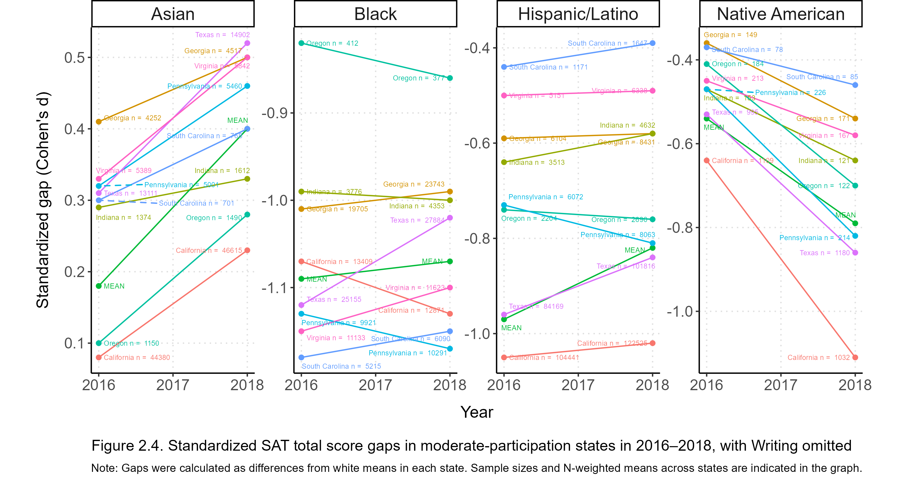
These graphs look very similar to the original ones. To discern more subtle patterns, below I reproduce the redesign effect tables from above, but now omitting the Writing section.
| National gaps in 2018 | Gaps in states with high participation | Gaps in states with moderate participation | ||||||||||
| Group | Observed | Predicted | Δ | Mean 2018 | Mean 2009–2016 | Δ | Mean 2018 | Mean 2016 | Δ | |||
|---|---|---|---|---|---|---|---|---|---|---|---|---|
| Asian/Pacific Islander | 0.50 | 0.31 | 0.19 | 0.49 | 0.29 | 0.20 | 0.40 | 0.18 | 0.22 | |||
| Group | Effect |
|---|---|
| Asian/Pacific Islander | 0.21 |
Comparing the estimated redesign effects in Tables 2.4 and 2.6, it can be seen that Asian, black, and Native American effects are essentially invariant whether two or three test sections are included. For Hispanics, there seems to be a slight attenuation of the gap due to the omission of the Writing section. However, the attenuation is not observed consistently across states, and the effect is mostly just due to Hispanics in Texas improving strongly in relation to whites–Texas with its large population gets a large weight in my calculations. Nor did the size of the white-Hispanic gap vary depending on the inclusion of Writing before 2017 in the national data (cf., Figure 1.5), so the apparent effect may be just a fluke. That there is no discernible effect for Asians, unlike in the national data, suggests that the removal of the Writing section accounts for only a small portion of the redesign effect at best.
In Chapter 1, I also found that after 2017 Asians made more gains in the verbal section (ERW) than the math section. To test if this was the case at the state level, too, I analyzed Asian verbal and math gains in the high- and moderate-participation states. The next figure shows this comparison. Where appropriate, the gaps were aggregated in line with the procedures explicated in [Note 13].
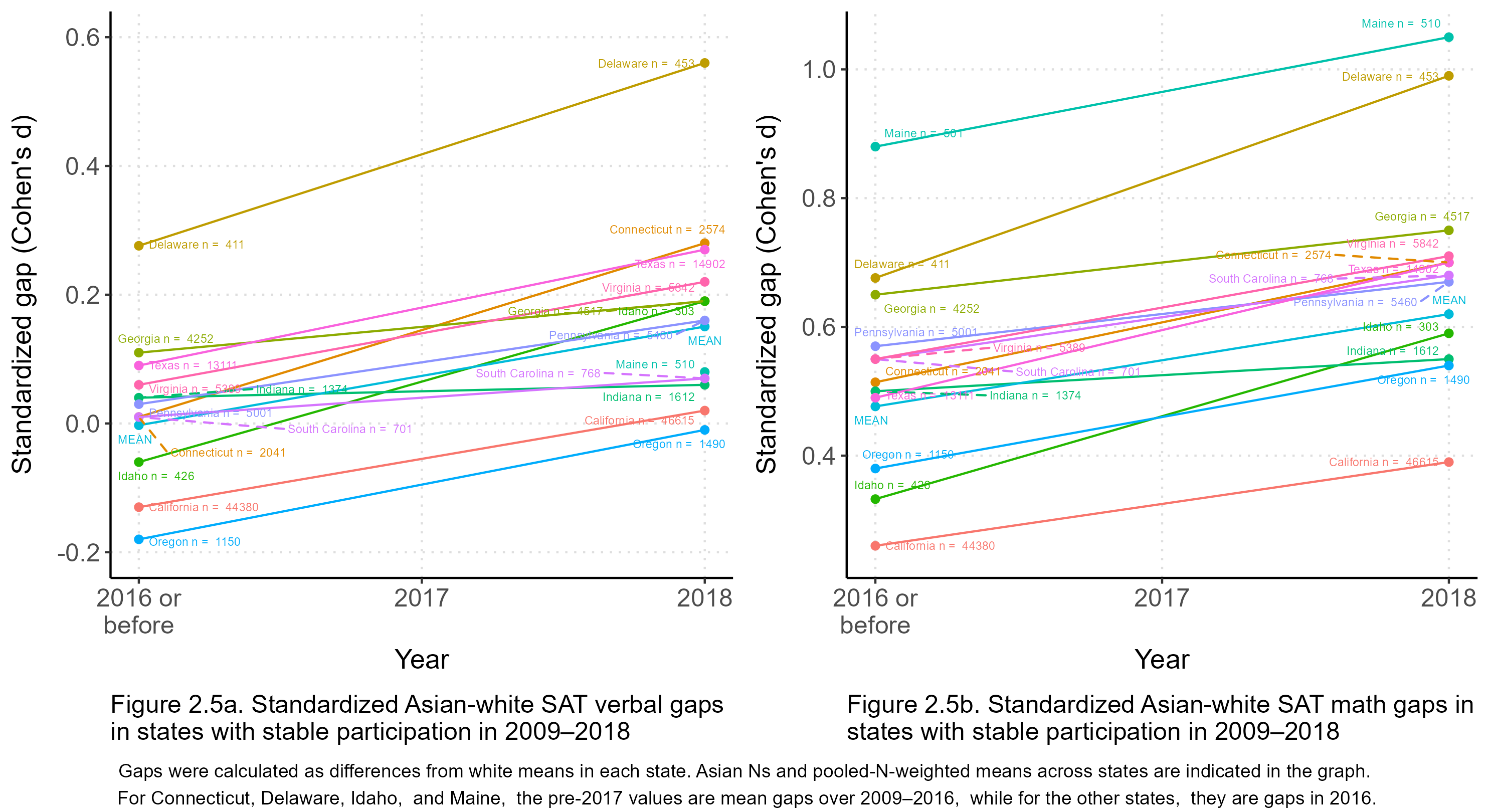
Interestingly, at the state level Asian gains were not verbally biased. On average, the gains were almost identical in both sections. The mean verbal gap across these states was d = 0 before 2017, rising to d = 0.15 in 2018, while the mean math gap increased from d = 0.48 to d = 0.62. The average verbal gain was d = 0.15, and the average math gain was d = 0.14. This finding is at variance with the national results, but I regard the state-level results as more reliable as they are much less confounded by selection bias. Therefore, it appears that the two sections contributed equally to the supernormal total score gains that Asians experienced after the new test was introduced.
The analysis presented in this chapter is based on results from dozens of SAT-taker cohorts from a number states. The sample sizes are large for almost all of the aggregate-level racial/ethnic comparisons, so random sampling error is unlikely to a major source of bias in the overall estimates. Nonetheless, the comparisons rely on various assumptions, which, if they do not actually hold, would vitiate the causal interpretations I have made. Aside from the assumptions discussed above, you could conjecture that there are more subtle confounds, too, such as moderation of the redesign effect by ability level. However, the patterns of results are so consistent across different states that I think my interpretations are reasonable. This is especially so in the case of Asian-Americans: with the 2017 redesign, something about how SAT items are written and scored changed in ways that played to their strengths. This does not seem to be just a one-off shift in the size of the Asian advantage, either, because Asians have been expanding their lead on whites in recent years much faster than they did historically.
Racial/ethnic SAT gaps in states with high participation in 2009–2018 (CSV)
Year,State,Group,N,Total_Mean,Total_SD,d,Participation_rate
2009,Connecticut,Asian/Pacific Islander,1621,1661,363,0.22,87%
2009,Connecticut,Black,3403,1250,273,-1.21,87%
2009,Connecticut,Hispanic/Latino,3015,1334,296,-0.91,87%
2009,Connecticut,Native American,132,1487,295,-0.38,87%
2009,Connecticut,No Response,1641,1494,370,-0.35,87%
2009,Connecticut,White,25062,1596,287,0,87%
2009,Maine,Asian/Pacific Islander,384,1468,333,0.19,91%
2009,Maine,Black,213,1255,322,-0.48,91%
2009,Maine,Hispanic/Latino,199,1303,316,-0.33,91%
2009,Maine,Native American,255,1225,283,-0.58,91%
2009,Maine,No Response,1077,1240,329,-0.53,91%
2009,Maine,White,12594,1407,316,0,91%
2010,Connecticut,Asian/Pacific Islander,1849,1665,361,0.23,88%
2010,Connecticut,Black,3613,1252,274,-1.22,88%
2010,Connecticut,Hispanic/Latino,3256,1330,293,-0.94,88%
2010,Connecticut,Native American,117,1465,304,-0.47,88%
2010,Connecticut,No Response,1702,1533,351,-0.23,88%
2010,Connecticut,White,24763,1598,284,0,88%
2010,Maine,Asian/Pacific Islander,462,1447,352,0.14,92%
2010,Maine,Black,290,1227,285,-0.56,92%
2010,Maine,Hispanic/Latino,226,1366,309,-0.12,92%
2010,Maine,Native American,198,1216,290,-0.59,92%
2010,Maine,No Response,901,1263,335,-0.44,92%
2010,Maine,White,13081,1404,317,0,92%
2011,Maine,Asian/Pacific Islander,480,1469,343,0.19,92%
2011,Maine,Black,299,1220,274,-0.6,92%
2011,Maine,Hispanic/Latino,236,1388,289,-0.07,92%
2011,Maine,Native American,176,1206,274,-0.65,92%
2011,Maine,No Response,932,1207,304,-0.64,92%
2011,Maine,White,12652,1409,314,0,92%
2012,Delaware,Asian/Pacific Islander,398,1601,373,0.48,98%
2012,Delaware,Black,2373,1179,257,-0.93,98%
2012,Delaware,Hispanic/Latino,697,1214,284,-0.78,98%
2012,Delaware,Native American,62,1361,309,-0.3,98%
2012,Delaware,No Response,282,1190,295,-0.85,98%
2012,Delaware,White,5661,1452,307,0,98%
2012,Maine,Asian/Pacific Islander,481,1510,342,0.32,92%
2012,Maine,Black,312,1194,293,-0.69,92%
2012,Maine,Hispanic/Latino,219,1360,330,-0.16,92%
2012,Maine,Native American,188,1210,280,-0.64,92%
2012,Maine,No Response,799,1197,312,-0.68,92%
2012,Maine,White,12580,1409,310,0,92%
2013,Delaware,Asian/Pacific Islander,365,1605,366,0.51,99%
2013,Delaware,Black,2382,1171,262,-0.95,99%
2013,Delaware,Hispanic/Latino,838,1199,281,-0.82,99%
2013,Delaware,Native American,47,1252,297,-0.64,99%
2013,Delaware,No Response,248,1196,306,-0.83,99%
2013,Delaware,White,5433,1448,305,0,99%
2013,Idaho,Asian/Pacific Islander,419,1433,347,0.09,97%
2013,Idaho,Black,214,1262,298,-0.5,97%
2013,Idaho,Hispanic/Latino,2060,1181,267,-0.79,97%
2013,Idaho,Native American,295,1270,281,-0.47,97%
2013,Idaho,No Response,1255,1259,291,-0.51,97%
2013,Idaho,White,12834,1406,287,0,97%
2013,Maine,Asian/Pacific Islander,575,1467,351,0.21,91%
2013,Maine,Black,329,1206,309,-0.61,91%
2013,Maine,Hispanic/Latino,230,1319,327,-0.26,91%
2013,Maine,Native American,202,1250,286,-0.48,91%
2013,Maine,No Response,960,1167,322,-0.74,91%
2013,Maine,White,12009,1401,318,0,91%
2014,Connecticut,Asian/Pacific Islander,2199,1670,363,0.23,85%
2014,Connecticut,Black,4042,1259,289,-1.2,85%
2014,Connecticut,Hispanic/Latino,4430,1321,314,-0.97,85%
2014,Connecticut,Native American,131,1433,269,-0.6,85%
2014,Connecticut,No Response,838,1311,350,-1.02,85%
2014,Connecticut,White,23710,1604,286,0,85%
2014,Delaware,Asian/Pacific Islander,429,1631,384,0.57,99%
2014,Delaware,Black,2362,1175,258,-0.92,99%
2014,Delaware,Hispanic/Latino,850,1225,290,-0.73,99%
2014,Delaware,Native American,41,1219,335,-0.74,99%
2014,Delaware,No Response,192,1202,309,-0.79,99%
2014,Delaware,White,5479,1450,313,0,99%
2014,Idaho,Asian/Pacific Islander,488,1444,339,0.13,92%
2014,Idaho,Black,259,1240,283,-0.59,92%
2014,Idaho,Hispanic/Latino,2167,1200,259,-0.74,92%
2014,Idaho,Native American,303,1223,256,-0.65,92%
2014,Idaho,No Response,1166,1233,278,-0.62,92%
2014,Idaho,White,13364,1406,280,0,92%
2014,Maine,Asian/Pacific Islander,601,1492,342,0.26,93%
2014,Maine,Black,377,1201,285,-0.67,93%
2014,Maine,Hispanic/Latino,220,1369,322,-0.13,93%
2014,Maine,Native American,188,1203,287,-0.67,93%
2014,Maine,No Response,885,1141,282,-0.87,93%
2014,Maine,White,11649,1411,313,0,93%
2015,Connecticut,Asian/Pacific Islander,2316,1680,363,0.26,87%
2015,Connecticut,Black,4275,1247,287,-1.25,87%
2015,Connecticut,Hispanic/Latino,2901,1338,320,-0.92,87%
2015,Connecticut,Native American,143,1359,306,-0.86,87%
2015,Connecticut,No Response,970,1290,358,-1.09,87%
2015,Connecticut,White,22920,1605,286,0,87%
2015,Delaware,Asian/Pacific Islander,443,1625,367,0.52,100%
2015,Delaware,Black,2457,1193,253,-0.96,100%
2015,Delaware,Hispanic/Latino,888,1233,272,-0.8,100%
2015,Delaware,Native American,51,1204,274,-0.88,100%
2015,Delaware,No Response,233,1158,279,-1.04,100%
2015,Delaware,White,5368,1468,299,0,100%
2015,Idaho,Asian/Pacific Islander,372,1472,351,0.09,92%
2015,Idaho,Black,175,1254,283,-0.7,92%
2015,Idaho,Hispanic/Latino,1654,1251,253,-0.72,92%
2015,Idaho,Native American,251,1257,255,-0.69,92%
2015,Idaho,No Response,4658,1250,246,-0.74,92%
2015,Idaho,White,10373,1448,277,0,92%
2015,Maine,Asian/Pacific Islander,521,1507,354,0.29,92%
2015,Maine,Black,407,1212,281,-0.64,92%
2015,Maine,Hispanic/Latino,229,1349,309,-0.21,92%
2015,Maine,Native American,167,1222,273,-0.61,92%
2015,Maine,No Response,929,1188,292,-0.72,92%
2015,Maine,White,11501,1414,317,0,92%
2016,Connecticut,Asian/Pacific Islander,2221,1666,359,0.25,86%
2016,Connecticut,Black,3988,1230,292,-1.25,86%
2016,Connecticut,Hispanic/Latino,5809,1284,316,-1.05,86%
2016,Connecticut,Native American,125,1362,338,-0.8,86%
2016,Connecticut,No Response,1517,1439,382,-0.52,86%
2016,Connecticut,White,21355,1592,288,0,86%
2016,Delaware,Asian/Pacific Islander,422,1574,382,0.4,100%
2016,Delaware,Black,2418,1180,265,-0.93,100%
2016,Delaware,Hispanic/Latino,1073,1232,284,-0.73,100%
2016,Delaware,Native American,54,1233,325,-0.72,100%
2016,Delaware,No Response,296,1259,309,-0.63,100%
2016,Delaware,White,5099,1451,303,0,100%
2016,Idaho,Asian/Pacific Islander,427,1426,334,0.07,90%
2016,Idaho,Black,257,1215,301,-0.67,90%
2016,Idaho,Hispanic/Latino,2395,1209,270,-0.7,90%
2016,Idaho,Native American,266,1166,255,-0.85,90%
2016,Idaho,No Response,1317,1272,294,-0.47,90%
2016,Idaho,White,12970,1406,284,0,90%
2018,Connecticut,All Groups,44700,1053,216,-0.28,100%
2018,Connecticut,Asian,2574,1216,221,0.53,100%
2018,Connecticut,Asian/Pacific Islander,2615,1211,224,0.5,100%
2018,Connecticut,Black,5241,904,171,-1.08,100%
2018,Connecticut,Female,22014,1058,206,-0.26,100%
2018,Connecticut,Hispanic/Latino,8928,934,193,-0.91,100%
2018,Connecticut,Male,22664,1049,223,-0.3,100%
2018,Connecticut,Native American,130,973,201,-0.7,100%
2018,Connecticut,Pacific Islander,41,918,199,-0.98,100%
2018,Connecticut,Two or More Races,1303,1092,215,-0.1,100%
2018,Connecticut,White,25555,1111,196,0,100%
2018,Delaware,All Groups,11055,998,205,-0.37,100%
2018,Delaware,Asian,453,1224,216,0.8,100%
2018,Delaware,Asian/Pacific Islander,465,1216,219,0.75,100%
2018,Delaware,Black,2361,909,159,-0.91,100%
2018,Delaware,Female,5490,1003,190,-0.37,100%
2018,Delaware,Hispanic/Latino,1467,928,168,-0.78,100%
2018,Delaware,Male,5553,993,210,-0.4,100%
2018,Delaware,Native American,69,906,165,-0.88,100%
2018,Delaware,Pacific Islander,12,928,115,-0.77,100%
2018,Delaware,Two or More Races,575,992,195,-0.42,100%
2018,Delaware,White,5114,1072,188,0,100%
2018,Idaho,All Groups,20484,1001,183,-0.21,100%
2018,Idaho,Asian,303,1112,207,0.4,100%
2018,Idaho,Asian/Pacific Islander,364,1086,210,0.26,100%
2018,Idaho,Black,194,912,167,-0.7,100%
2018,Idaho,Female,10067,1005,178,-0.19,100%
2018,Idaho,Hispanic/Latino,2943,925,161,-0.64,100%
2018,Idaho,Male,10408,998,193,-0.22,100%
2018,Idaho,Native American,281,896,159,-0.79,100%
2018,Idaho,Pacific Islander,61,958,177,-0.45,100%
2018,Idaho,Two or More Races,579,1049,175,0.06,100%
2018,Idaho,White,12837,1039,182,0,100%
2018,Maine,All Groups,14310,1013,204,-0.18,99%
2018,Maine,Asian,510,1164,207,0.61,99%
2018,Maine,Asian/Pacific Islander,515,1164,207,0.61,99%
2018,Maine,Black,393,907,164,-0.75,99%
2018,Maine,Female,6899,1021,189,-0.14,99%
2018,Maine,Hispanic/Latino,354,1007,187,-0.22,99%
2018,Maine,Male,7409,1006,207,-0.21,99%
2018,Maine,Native American,162,904,166,-0.77,99%
2018,Maine,Pacific Islander,5,NA,NA,NA,99%
2018,Maine,Two or More Races,372,1045,181,-0.02,99%
2018,Maine,White,9890,1048,188,0,99%
Racial/ethnic SAT gaps in states with moderate participation in 2016–2018 (CSV)
Year,State,Group,N,Total_Mean,Total_SD,Total_d
2016,California,All Groups,241589,1476,323,-0.47
2016,California,Asian,44380,1638,346,0.04
2016,California,Black,13409,1320,283,-1.07
2016,California,Hispanic/Latino,104441,1332,266,-1.07
2016,California,Native American,1109,1433,291,-0.67
2016,California,No Response,8191,1502,353,-0.42
2016,California,Other,2794,1613,350,-0.04
2016,California,Pacific Islander,590,1330,281,-1.03
2016,California,Two or More Races,5262,1543,302,-0.28
2016,California,White,61413,1624,285,0
2016,Georgia,All Groups,65473,1459,297,-0.32
2016,Georgia,Asian,4252,1658,347,0.38
2016,Georgia,Black,19705,1285,254,-1.01
2016,Georgia,Hispanic/Latino,6104,1389,263,-0.6
2016,Georgia,Native American,149,1456,297,-0.35
2016,Georgia,No Response,1431,1423,316,-0.47
2016,Georgia,Other,555,1564,317,0.05
2016,Georgia,Pacific Islander,24,1302,NA,NA
2016,Georgia,Two or More Races,1289,1449,271,-0.38
2016,Georgia,White,31964,1551,270,0
2016,Indiana,All Groups,44333,1472,278,-0.13
2016,Indiana,Asian,1374,1579,368,0.26
2016,Indiana,Black,3776,1253,247,-0.97
2016,Indiana,Hispanic/Latino,3513,1341,260,-0.63
2016,Indiana,Native American,153,1387,248,-0.46
2016,Indiana,No Response,818,1453,303,-0.21
2016,Indiana,Other,380,1471,304,-0.14
2016,Indiana,Pacific Islander,7,1337,NA,NA
2016,Indiana,Two or More Races,822,1437,261,-0.27
2016,Indiana,White,33490,1508,264,0
2016,MEAN,Asian,75358,NA,NA,0.22
2016,MEAN,Black,88726,NA,NA,-1.08
2016,MEAN,Hispanic/Latino,212825,NA,NA,-0.86
2016,MEAN,Native American,3107,NA,NA,-0.51
2016,MEDIAN,Asian,NA,NA,NA,0.28
2016,MEDIAN,Black,NA,NA,NA,-1.09
2016,MEDIAN,Hispanic/Latino,NA,NA,NA,-0.68
2016,MEDIAN,Native American,NA,NA,NA,-0.46
2016,Oregon,All Groups,16703,1545,291,-0.12
2016,Oregon,Asian,1150,1596,330,0.06
2016,Oregon,Black,412,1362,281,-0.79
2016,Oregon,Hispanic/Latino,2204,1376,263,-0.74
2016,Oregon,Native American,184,1456,269,-0.45
2016,Oregon,No Response,566,1571,320,-0.03
2016,Oregon,Other,123,1614,317,0.13
2016,Oregon,Pacific Islander,36,1380,256,-0.72
2016,Oregon,Two or More Races,472,1536,274,-0.16
2016,Oregon,White,11156,1579,275,0
2016,Pennsylvania,All Groups,92569,1487,301,-0.17
2016,Pennsylvania,Asian,5001,1618,373,0.29
2016,Pennsylvania,Black,9921,1228,272,-1.12
2016,Pennsylvania,Hispanic/Latino,6072,1333,294,-0.73
2016,Pennsylvania,Native American,226,1403,293,-0.48
2016,Pennsylvania,No Response,2701,1431,330,-0.38
2016,Pennsylvania,Other,749,1512,345,-0.08
2016,Pennsylvania,Pacific Islander,23,1423,NA,NA
2016,Pennsylvania,Two or More Races,1321,1425,289,-0.4
2016,Pennsylvania,White,66555,1535,274,0
2016,South Carolina,All Groups,22324,1458,285,-0.29
2016,South Carolina,Asian,701,1601,338,0.24
2016,South Carolina,Black,5215,1237,232,-1.18
2016,South Carolina,Hispanic/Latino,1171,1420,263,-0.45
2016,South Carolina,Native American,78,1429,286,-0.41
2016,South Carolina,No Response,398,1443,310,-0.36
2016,South Carolina,Other,139,1496,285,-0.16
2016,South Carolina,Pacific Islander,14,1400,NA,NA
2016,South Carolina,Two or More Races,505,1442,266,-0.36
2016,South Carolina,White,14103,1537,262,0
2016,Texas,All Groups,196028,1393,316,-0.52
2016,Texas,Asian,13111,1641,354,0.29
2016,Texas,Black,25155,1245,270,-1.11
2016,Texas,Hispanic/Latino,84169,1286,274,-0.97
2016,Texas,Native American,995,1400,298,-0.55
2016,Texas,No Response,5944,1256,343,-1.04
2016,Texas,Other,1587,1461,353,-0.33
2016,Texas,Pacific Islander,100,1363,311,-0.68
2016,Texas,Two or More Races,2311,1458,283,-0.34
2016,Texas,White,62656,1554,282,0
2016,Virginia,All Groups,57861,1535,303,-0.23
2016,Virginia,Asian,5389,1689,332,0.31
2016,Virginia,Black,11133,1295,257,-1.15
2016,Virginia,Hispanic/Latino,5151,1465,276,-0.51
2016,Virginia,Native American,213,1483,281,-0.44
2016,Virginia,No Response,1669,1549,326,-0.2
2016,Virginia,Other,709,1564,311,-0.14
2016,Virginia,Pacific Islander,41,1481,313,-0.45
2016,Virginia,Two or More Races,1644,1506,288,-0.36
2016,Virginia,White,31912,1603,272,0
2018,California,All Groups,262228,1076,206,-0.45
2018,California,Asian,46615,1210,202,0.23
2018,California,Black,12871,967,170,-1.13
2018,California,Female,142745,1061,197,-0.55
2018,California,Hispanic/Latino,122525,990,171,-1.02
2018,California,Male,119474,1093,212,-0.37
2018,California,Native American,1032,969,184,-1.11
2018,California,Pacific Islander,1323,1020,172,-0.82
2018,California,Two or More Races,11415,1158,195,-0.05
2018,California,White,59845,1167,179,0
2018,Georgia,All Groups,74240,1064,185,-0.35
2018,Georgia,Asian,4517,1212,203,0.5
2018,Georgia,Black,23743,965,157,-0.99
2018,Georgia,Female,41217,1053,179,-0.42
2018,Georgia,Hispanic/Latino,8431,1029,163,-0.58
2018,Georgia,Male,33011,1079,190,-0.26
2018,Georgia,Native American,171,1035,170,-0.54
2018,Georgia,Pacific Islander,71,1053,148,-0.44
2018,Georgia,Two or More Races,2730,1088,172,-0.23
2018,Georgia,White,33027,1126,167,0
2018,Indiana,All Groups,48962,1086,170,-0.14
2018,Indiana,Asian,1612,1164,207,0.33
2018,Indiana,Black,4353,948,146,-1
2018,Indiana,Female,26975,1071,164,-0.24
2018,Indiana,Hispanic/Latino,4632,1016,165,-0.58
2018,Indiana,Male,21980,1104,178,-0.04
2018,Indiana,Native American,121,1005,152,-0.64
2018,Indiana,Pacific Islander,29,1116,151,0.04
2018,Indiana,Two or More Races,1788,1079,167,-0.19
2018,Indiana,White,35610,1110,163,0
2018,MEAN,Asian,81206,NA,NA,0.4
2018,MEAN,Black,97232,NA,NA,-1.07
2018,MEAN,Hispanic/Latino,256142,NA,NA,-0.82
2018,MEAN,Native American,3092,NA,NA,-0.79
2018,MEDIAN,Asian,NA,NA,NA,0.43
2018,MEDIAN,Black,NA,NA,NA,-1.06
2018,MEDIAN,Hispanic/Latino,NA,NA,NA,-0.67
2018,MEDIAN,Native American,NA,NA,NA,-0.67
2018,Oregon,All Groups,17476,1117,179,-0.13
2018,Oregon,Asian,1490,1188,198,0.28
2018,Oregon,Black,377,995,169,-0.86
2018,Oregon,Female,9857,1098,173,-0.25
2018,Oregon,Hispanic/Latino,2690,1012,166,-0.76
2018,Oregon,Male,7617,1142,186,0.01
2018,Oregon,Native American,122,1022,133,-0.7
2018,Oregon,Pacific Islander,90,1015,177,-0.74
2018,Oregon,Two or More Races,1054,1134,175,-0.04
2018,Oregon,White,11134,1140,169,0
2018,Pennsylvania,All Groups,96740,1086,188,-0.19
2018,Pennsylvania,Asian,5460,1198,211,0.46
2018,Pennsylvania,Black,10291,923,172,-1.17
2018,Pennsylvania,Female,52109,1072,179,-0.28
2018,Pennsylvania,Hispanic/Latino,8063,984,181,-0.81
2018,Pennsylvania,Male,44616,1102,192,-0.1
2018,Pennsylvania,Native American,214,983,149,-0.82
2018,Pennsylvania,Pacific Islander,73,1033,160,-0.52
2018,Pennsylvania,Two or More Races,3199,1078,188,-0.25
2018,Pennsylvania,White,66836,1120,167,0
2018,South Carolina,All Groups,25390,1070,177,-0.28
2018,South Carolina,Asian,768,1186,196,0.4
2018,South Carolina,Black,6090,938,142,-1.15
2018,South Carolina,Female,14338,1059,174,-0.36
2018,South Carolina,Hispanic/Latino,1647,1055,166,-0.39
2018,South Carolina,Male,11045,1085,186,-0.2
2018,South Carolina,Native American,85,1043,157,-0.46
2018,South Carolina,Pacific Islander,25,1033,136,-0.52
2018,South Carolina,Two or More Races,1064,1086,169,-0.2
2018,South Carolina,White,15307,1119,164,0
2018,Texas,All Groups,226374,1032,198,-0.46
2018,Texas,Asian,14902,1215,201,0.52
2018,Texas,Black,27884,942,170,-1.02
2018,Texas,Female,119684,1026,187,-0.51
2018,Texas,Hispanic/Latino,101816,973,172,-0.84
2018,Texas,Male,106619,1039,211,-0.41
2018,Texas,Native American,1180,967,184,-0.86
2018,Texas,Pacific Islander,317,1010,170,-0.62
2018,Texas,Two or More Races,5901,1095,189,-0.14
2018,Texas,White,69127,1120,177,0
2018,Virginia,All Groups,61576,1117,188,-0.22
2018,Virginia,Asian,5842,1241,193,0.5
2018,Virginia,Black,11623,975,158,-1.1
2018,Virginia,Female,32821,1104,185,-0.3
2018,Virginia,Hispanic/Latino,6338,1074,175,-0.49
2018,Virginia,Male,28754,1132,193,-0.13
2018,Virginia,Native American,167,1060,155,-0.58
2018,Virginia,Pacific Islander,68,1099,164,-0.34
2018,Virginia,Two or More Races,3576,1119,183,-0.22
2018,Virginia,White,32692,1156,167,0
R code for states with high or moderate participation in 2009–2018
# packages that may be used
# uncomment if you don't have these installed already

#install.packages("fitdistrplus")
#install.packages("ztable")
#install.packages("reshape2")
#install.packages("ggplot2")
#install.packages("ggrepel")
#install.packages("tigerstats")
#install.packages("sjPlot")
#install.packages("scales")
#install.packages("gridExtra")
#install.packahes("grid")

# read pre-2017 high participation data
high_participation_pre_2017 <- read.csv(text="Year,State,HS_graduates,SAT_takers,Participation_rate
2009,Connecticut,41201,35799,0.87
2009,Maine,16455,14954,0.91
2010,Connecticut,40996,36076,0.88
2010,Maine,16708,15383,0.92
2011,Maine,16254,14975,0.92
2012,Delaware,10015,9838,0.98
2012,Maine,16141,14799,0.92
2013,Delaware,9759,9669,0.99
2013,Idaho,17830,17352,0.97
2013,Maine,15860,14501,0.91
2014,Connecticut,42968,36370,0.85
2014,Delaware,9829,9727,0.99
2014,Idaho,19562,18078,0.92
2014,Maine,15227,14118,0.93
2015,Connecticut,41956,36445,0.87
2015,Delaware,9744,9823,1.01
2015,Idaho,19304,17695,0.92
2015,Maine,15125,13936,0.92
2016,Connecticut,41529,35902,0.86
2016,Delaware,9509,9772,1.03
2016,Idaho,19915,17950,0.9")

library(scales)
high_participation_pre_2017<-with(high_participation_pre_2017, rbind(high_participation_pre_2017,list("Total", "", sum(HS_graduates), sum(SAT_takers), round(sum(SAT_takers)/sum(HS_graduates),2))))
high_participation_pre_2017$Participation_rate <- percent(high_participation_pre_2017$Participation_rate)
colnames(high_participation_pre_2017) <- gsub("_", " ", colnames(high_participation_pre_2017))

# html table of pre-2017 high-participation states
library("ztable")
high_participation_pre_2017_table <- ztable(high_participation_pre_2017,zebra=2,zebra.color="#d4effc;", caption="Table 2.1. High-participation states in 2009–2016", caption.placement="top",caption.position="l", caption.bold=TRUE, align="rlrrr",include.rownames=FALSE,size=3,colnames.bold=TRUE)
high_participation_pre_2017_table <- hlines(high_participation_pre_2017_table, add = c(21))
capture.output(high_participation_pre_2017_table,file="table2_1.html")

# read pre-2017 high participation state data
high_participation_pre_2017_data <- read.csv(text="Year,State,Group,N,Verbal_Mean,Verbal_SD,Math_Mean,Math_SD,Writing_Mean,Writing_SD
2009,Connecticut,Native American,132,502,109,493,107,492,102
2009,Connecticut,Asian/Pacific Islander,1621,529,129,590,131,542,132
2009,Connecticut,Black,3403,419,98,410,100,421,97
2009,Connecticut,Mexican,197,472,103,476,114,474,105
2009,Connecticut,Puerto Rican,1301,428,100,420,100,432,97
2009,Connecticut,Other Hispanic/Latino,1517,457,110,455,111,459,112
2009,Connecticut,White,25062,530,103,534,105,532,102
2009,Connecticut,Other,925,479,123,476,123,484,119
2009,Connecticut,No Response,1641,502,134,496,134,496,131
2009,Connecticut,All Groups,35799,509,113,513,117,512,112
2010,Connecticut,Native American,117,490,112,482,111,493,105
2010,Connecticut,Asian/Pacific Islander,1849,531,127,589,131,545,132
2010,Connecticut,Black,3613,420,99,411,101,421,96
2010,Connecticut,Mexican,227,470,105,469,110,468,104
2010,Connecticut,Puerto Rican,1451,425,98,420,99,426,96
2010,Connecticut,Other Hispanic/Latino,1578,456,107,459,109,460,110
2010,Connecticut,White,24763,530,101,534,105,534,101
2010,Connecticut,Other,776,487,124,484,125,493,123
2010,Connecticut,No Response,1702,514,126,509,127,510,126
2010,Connecticut,All Groups,36076,509,112,514,117,513,112
2014,Connecticut,Native American,131,475,95,477,98,481,97
2014,Connecticut,Asian/Pacific Islander,2199,532,129,590,130,548,133
2014,Connecticut,Black,4042,423,106,413,105,423,101
2014,Connecticut,Mexican,360,463,114,464,114,463,111
2014,Connecticut,Puerto Rican,1754,419,106,410,109,419,99
2014,Connecticut,Other Hispanic/Latino,2316,455,115,455,120,457,112
2014,Connecticut,White,23710,534,101,536,107,534,101
2014,Connecticut,Other,102,506,129,507,132,504,128
2014,Connecticut,No Response,838,442,127,433,126,436,125
2014,Connecticut,All Groups,3637,507,115,510,122,508,115
2015,Connecticut,Native American,143,461,111,445,115,453,104
2015,Connecticut,Asian/Pacific Islander,2316,539,129,594,130,547,133
2015,Connecticut,Black,4275,420,105,408,104,419,101
2015,Connecticut,Mexican,395,449,119,446,118,447,110
2015,Connecticut,Puerto Rican,213,419,104,405,105,414,102
2015,Connecticut,Other Hispanic/Latino,2293,449,115,448,119,449,113
2015,Connecticut,White,22920,535,101,536,107,534,101
2015,Connecticut,Other,1003,484,128,484,137,485,131
2015,Connecticut,No Response,970,435,132,428,128,427,126
2015,Connecticut,All Groups,36445,504,117,506,124,504,117
2016,Connecticut,Native American,125,462,121,444,125,456,119
2016,Connecticut,Asian,2206,536,127,590,131,543,130
2016,Connecticut,Black,3988,416,107,402,107,412,101
2016,Connecticut,Pacific Islander,15,371,NA,370,NA,346,NA
2016,Connecticut,Hispanic/Latino,5809,431,113,425,117,428,111
2016,Connecticut,White,21355,532,102,532,108,528,101
2016,Connecticut,Two or More Races,579,506,110,490,123,495,110
2016,Connecticut,Other,308,514,142,508,150,507,136
2016,Connecticut,No Response,1517,484,137,478,142,477,134
2016,Connecticut,All Groups,35902,500,118,500,126,497,117
2012,Delaware,Native American,62,455,110,463,110,443,114
2012,Delaware,Asian/Pacific Islander,398,519,134,561,134,521,135
2012,Delaware,Black,2373,396,95,399,92,384,90
2012,Delaware,Mexican,238,398,92,412,89,383,90
2012,Delaware,Puerto Rican,213,404,104,410,95,393,95
2012,Delaware,Other Hispanic/Latino,246,412,121,425,113,402,113
2012,Delaware,White,5661,486,111,492,109,474,111
2012,Delaware,Other,365,438,108,440,107,425,110
2012,Delaware,No Response,282,403,112,401,100,386,106
2012,Delaware,All Groups,9838,456,116,462,115,444,115
2013,Delaware,Native American,47,415,109,429,109,408,103
2013,Delaware,Asian/Pacific Islander,365,515,136,572,127,518,132
2013,Delaware,Black,2382,390,98,395,96,386,89
2013,Delaware,Mexican,303,390,92,404,91,391,82
2013,Delaware,Puerto Rican,279,404,106,394,94,393,91
2013,Delaware,Other Hispanic/Latino,256,406,116,415,117,401,116
2013,Delaware,White,5433,484,111,489,109,475,109
2013,Delaware,Other,356,433,118,432,114,426,114
2013,Delaware,No Response,248,405,118,398,111,393,101
2013,Delaware,All Groups,9669,451,118,457,117,443,113
2014,Delaware,Native American,41,421,117,403,118,395,126
2014,Delaware,Asian/Pacific Islander,429,527,133,571,139,533,143
2014,Delaware,Black,2362,395,96,396,93,384,90
2014,Delaware,Mexican,325,395,94,413,85,386,89
2014,Delaware,Puerto Rican,230,406,102,408,98,399,92
2014,Delaware,Other Hispanic/Latino,295,422,126,433,120,414,120
2014,Delaware,White,5479,487,114,489,112,474,112
2014,Delaware,Other,374,433,116,430,111,419,111
2014,Delaware,No Response,192,405,110,406,109,391,114
2014,Delaware,All Groups,9727,456,119,459,118,444,117
2015,Delaware,Native American,51,413,94,401,99,390,103
2015,Delaware,Asian/Pacific Islander,443,529,129,572,129,524,138
2015,Delaware,Black,2457,405,93,400,90,388,90
2015,Delaware,Mexican,333,404,95,409,88,390,91
2015,Delaware,Puerto Rican,241,420,103,415,100,404,95
2015,Delaware,Other Hispanic/Latino,314,425,106,422,98,412,100
2015,Delaware,White,5368,496,106,494,107,478,110
2015,Delaware,Other,383,436,109,423,107,414,107
2015,Delaware,No Response,233,389,107,395,98,374,96
2015,Delaware,All Groups,9823,462,113,461,114,445,115
2016,Delaware,Native American,54,429,123,404,108,400,120
2016,Delaware,Asian,417,511,133,552,144,515,135
2016,Delaware,Black,2418,403,98,392,96,385,92
2016,Delaware,Pacific Islander,5,462,NA,394,NA,440,NA
2016,Delaware,Hispanic/Latino,1073,417,105,415,100,400,101
2016,Delaware,White,5099,492,110,487,108,472,109
2016,Delaware,Two or More Races,158,475,92,463,94,450,92
2016,Delaware,Other,252,428,116,408,110,406,113
2016,Delaware,No Response,296,435,115,417,111,407,108
2016,Delaware,All Groups,9772,458,116,453,116,440,113
2013,Idaho,Native American,295,424,106,424,103,422,94
2013,Idaho,Asian/Pacific Islander,419,463,125,510,134,460,116
2013,Idaho,Black,214,423,117,413,106,426,99
2013,Idaho,Mexican,1303,388,95,395,97,394,83
2013,Idaho,Puerto Rican,26,440,130,451,106,447,106
2013,Idaho,Other Hispanic/Latino,731,389,108,396,104,399,95
2013,Idaho,White,12834,469,106,473,107,464,97
2013,Idaho,Other,275,436,121,430,113,433,106
2013,Idaho,No Response,1255,420,112,422,104,417,98
2013,Idaho,All Groups,17352,454,110,459,111,451,100
2014,Idaho,Native American,303,414,99,409,91,400,86
2014,Idaho,Asian/Pacific Islander,488,474,123,503,129,467,114
2014,Idaho,Black,259,416,108,407,99,417,98
2014,Idaho,Mexican,1394,402,93,399,91,399,89
2014,Idaho,Puerto Rican,29,443,112,434,95,432,89
2014,Idaho,Other Hispanic/Latino,744,399,100,399,96,398,95
2014,Idaho,White,13364,473,104,470,103,463,95
2014,Idaho,Other,331,455,113,447,107,439,109
2014,Idaho,No Response,1166,416,106,411,99,406,95
2014,Idaho,All Groups,18078,458,107,456,106,450,99
2015,Idaho,Native American,251,432,98,428,88,397,89
2015,Idaho,Asian/Pacific Islander,372,485,128,521,130,466,121
2015,Idaho,Black,175,421,107,418,103,415,95
2015,Idaho,Mexican,1091,418,93,420,89,407,85
2015,Idaho,Puerto Rican,33,468,103,444,84,444,100
2015,Idaho,Other Hispanic/Latino,530,423,97,417,95,413,90
2015,Idaho,White,10373,493,103,488,100,467,96
2015,Idaho,Other,212,476,112,475,111,453,101
2015,Idaho,No Response,4658,427,95,422,88,401,82
2015,Idaho,All Groups,17695,467,106,463,103,442,98
2016,Idaho,Native American,266,396,96,392,96,378,83
2016,Idaho,Asian,418,468,119,501,127,458,115
2016,Idaho,Black,257,416,114,393,106,406,105
2016,Idaho,Pacific Islander,9,480,NA,506,NA,433,NA
2016,Idaho,Hispanic/Latino,2395,409,102,401,99,399,90
2016,Idaho,White,12970,480,107,466,103,460,97
2016,Idaho,Two or More Races,69,527,103,522,90,504,94
2016,Idaho,Other,249,445,118,429,115,430,104
2016,Idaho,No Response,1317,436,113,423,105,413,99
2016,Idaho,All Groups,1795,465,111,453,107,446,100
2009,Maine,Native American,255,414,103,418,105,393,98
2009,Maine,Asian/Pacific Islander,384,449,110,566,134,453,116
2009,Maine,Black,213,430,121,415,114,410,112
2009,Maine,Mexican,64,437,131,428,111,413,112
2009,Maine,Puerto Rican,38,425,110,419,110,407,113
2009,Maine,Other Hispanic/Latino,97,457,115,441,111,442,104
2009,Maine,White,12594,474,115,471,111,462,115
2009,Maine,Other,232,474,124,447,113,448,118
2009,Maine,No Response,1077,425,122,413,113,402,120
2009,Maine,All Groups,14954,468,116,467,114,455,116
2010,Maine,Native American,198,411,105,408,103,397,105
2010,Maine,Asian/Pacific Islander,462,441,122,557,136,449,122
2010,Maine,Black,290,421,107,402,97,404,103
2010,Maine,Mexican,64,468,112,466,103,450,118
2010,Maine,Puerto Rican,56,452,108,432,92,430,101
2010,Maine,Other Hispanic/Latino,106,469,114,458,116,455,115
2010,Maine,White,13081,474,114,470,112,460,116
2010,Maine,Other,225,454,121,437,111,433,118
2010,Maine,No Response,901,432,124,421,116,410,122
2010,Maine,All Groups,15383,468,115,467,115,454,117
2011,Maine,Native American,176,409,106,408,94,389,96
2011,Maine,Asian/Pacific Islander,480,441,116,573,132,455,122
2011,Maine,Black,299,415,105,405,96,400,95
2011,Maine,Mexican,54,465,110,458,94,447,95
2011,Maine,Puerto Rican,51,457,98,432,97,431,99
2011,Maine,Other Hispanic/Latino,131,480,99,479,114,463,105
2011,Maine,White,12652,477,114,472,110,460,115
2011,Maine,Other,200,463,127,470,122,440,135
2011,Maine,No Response,932,415,115,404,105,388,108
2011,Maine,All Groups,14975,469,116,469,114,453,116
2012,Maine,Native American,188,413,100,411,96,386,106
2012,Maine,Asian/Pacific Islander,481,453,119,586,122,471,128
2012,Maine,Black,312,405,103,398,106,391,107
2012,Maine,Mexican,47,456,105,443,119,441,126
2012,Maine,Puerto Rican,54,454,117,445,123,432,119
2012,Maine,Other Hispanic/Latino,118,458,123,474,109,448,121
2012,Maine,White,12580,477,109,474,111,458,115
2012,Maine,Other,220,459,130,470,121,443,127
2012,Maine,No Response,799,409,115,406,109,382,113
2012,Maine,All Groups,14799,470,112,472,115,452,117
2013,Maine,Native American,202,423,108,416,95,411,105
2013,Maine,Asian/Pacific Islander,575,442,121,570,135,455,123
2013,Maine,Black,329,408,116,400,109,398,109
2013,Maine,Mexican,54,435,115,443,97,402,98
2013,Maine,Puerto Rican,57,430,105,425,128,423,111
2013,Maine,Other Hispanic/Latino,119,463,129,457,122,436,118
2013,Maine,White,12009,471,115,471,114,459,114
2013,Maine,Other,196,463,130,468,119,454,126
2013,Maine,No Response,960,392,120,397,114,378,113
2013,Maine,All Groups,14501,462,118,467,118,451,116
2014,Maine,Native American,188,410,104,410,102,383,104
2014,Maine,Asian/Pacific Islander,601,448,115,580,130,464,124
2014,Maine,Black,377,410,105,398,104,393,99
2014,Maine,Mexican,46,465,138,449,125,441,133
2014,Maine,Puerto Rican,49,472,95,454,112,448,100
2014,Maine,Other Hispanic/Latino,125,462,122,461,108,449,114
2014,Maine,White,11649,477,112,476,112,458,114
2014,Maine,Other,198,463,114,453,125,441,118
2014,Maine,No Response,885,390,106,389,100,362,98
2014,Maine,All Groups,14118,467,114,471,117,449,116
2015,Maine,Native American,167,413,107,418,95,391,93
2015,Maine,Asian/Pacific Islander,521,462,123,573,129,472,130
2015,Maine,Black,407,411,106,405,99,396,98
2015,Maine,Mexican,50,464,108,451,103,443,108
2015,Maine,Puerto Rican,47,426,91,419,94,405,88
2015,Maine,Other Hispanic/Latino,132,467,120,471,117,442,115
2015,Maine,White,11501,477,116,478,113,459,113
2015,Maine,Other,182,466,124,455,107,442,113
2015,Maine,No Response,929,405,110,401,103,382,102
2015,Maine,All Groups,13936,468,117,473,116,451,115")

# combine Hispanics/Latinos

# Function for calculating the SD of a Gaussian mixture. 'ns' is a vector of subpopulation sample sizes, 'sds' is a vector of subpopulation SDs, and
# 'means' is a vector of subpopulation means.
gaussian_mixture_sd <- function(ns, sds, means) {
variance <- sum(sapply(1:length(sds), function(i) ns[i]/sum(ns)*(sds[i]^2 + means[i]^2))) - weighted.mean(means, ns)^2
return(round(sqrt(variance),0))
}

hispanic_data <- subset(high_participation_pre_2017_data, Group %in% c("Mexican", "Puerto Rican", "Other Hispanic/Latino"))
hispanic_combined <- data.frame(matrix(ncol = 10, nrow = 18))
colnames(hispanic_combined) <- colnames(high_participation_pre_2017_data)
hispanic_combined$Group <- "Hispanic/Latino"

j <- 1
for(i in seq(1, 54, 3)) {
hispanic_combined[j,"State"] <- hispanic_data[i,"State"]
hispanic_combined[j,"Year"] <- hispanic_data[i,"Year"]
hispanic_combined[j,"N"] <- sum(hispanic_data[c(i,i+1,i+2),"N"])
hispanic_combined[j,"Verbal_Mean"] <- round(with(hispanic_data, weighted.mean(Verbal_Mean[c(i,i+1,i+2)], N[c(i,i+1,i+2)])),0)
hispanic_combined[j,"Math_Mean"] <- round(with(hispanic_data, weighted.mean(Math_Mean[c(i,i+1,i+2)], N[c(i,i+1,i+2)])),0)
hispanic_combined[j,"Writing_Mean"] <- round(with(hispanic_data, weighted.mean(Writing_Mean[c(i,i+1,i+2)], N[c(i,i+1,i+2)])),0)
hispanic_combined[j,"Verbal_SD"] <- with(hispanic_data, gaussian_mixture_sd(N[c(i,i+1,i+2)], Verbal_SD[c(i,i+1,i+2)], Verbal_Mean[c(i,i+1,i+2)]))
hispanic_combined[j,"Math_SD"] <- with(hispanic_data, gaussian_mixture_sd(N[c(i,i+1,i+2)], Math_SD[c(i,i+1,i+2)], Math_Mean[c(i,i+1,i+2)]))
hispanic_combined[j,"Writing_SD"] <- with(hispanic_data, gaussian_mixture_sd(N[c(i,i+1,i+2)], Writing_SD[c(i,i+1,i+2)], Writing_Mean[c(i,i+1,i+2)]))

j <- j + 1
}

# add the combined Hispanic/Latino group to data
high_participation_pre_2017_data <- rbind(high_participation_pre_2017_data,hispanic_combined)

# add Asian/Pacific Islander group for 2016
aapi_data <- subset(high_participation_pre_2017_data, Group %in% c("Asian", "Pacific Islander"))
aapi_combined <- data.frame(matrix(ncol = 10, nrow = 3))
colnames(aapi_combined) <- colnames(high_participation_pre_2017_data)
aapi_combined$Group <- "Asian/Pacific Islander"

j <- 1
for(i in seq(1, 6, 2)) {
aapi_combined[j,"State"] <- aapi_data[i,"State"]
aapi_combined[j,"Year"] <- aapi_data[i,"Year"]
aapi_combined[j,"N"] <- sum(aapi_data[c(i,i+1),"N"])
aapi_combined[j,"Verbal_Mean"] <- round(with(aapi_data, weighted.mean(Verbal_Mean[c(i,i+1)], N[c(i,i+1)])),0)
aapi_combined[j,"Math_Mean"] <- round(with(aapi_data, weighted.mean(Math_Mean[c(i,i+1)], N[c(i,i+1)])),0)
aapi_combined[j,"Writing_Mean"] <- round(with(aapi_data, weighted.mean(Writing_Mean[c(i,i+1)], N[c(i,i+1)])),0)
aapi_combined[j,"Verbal_SD"] <- aapi_data$Verbal_SD[i]
aapi_combined[j,"Math_SD"] <- aapi_data$Math_SD[i]
aapi_combined[j,"Writing_SD"] <- aapi_data$Writing_SD[i]

j <- j + 1
}

# add the combined Asian/Pacific Islander group to data
high_participation_pre_2017_data <- rbind(high_participation_pre_2017_data,aapi_combined)

# calculate total score means and SDs
high_participation_pre_2017_data$Total_Mean <- with(high_participation_pre_2017_data, Verbal_Mean+Math_Mean+Writing_Mean)
high_participation_pre_2017_data$Total_SD <- round(sqrt(with(high_participation_pre_2017_data, Verbal_SD^2 + Math_SD^2 + Writing_SD^2 + 2 * 0.759 * Verbal_SD * Math_SD + 2 * 0.839 * Verbal_SD * Writing_SD + 2 * 0.764 * Math_SD * Writing_SD)),0)

# calculate standardized gaps for pre-2017 high-participation states

# function for calculating gaps
cohen_d <- function(group1_mean, group1_sd, group1_N, group2_mean, group2_sd, group2_N)  {
s <- sqrt( ( (group1_N-1)*group1_sd^2 + (group2_N-1)*group2_sd^2 ) / (group1_N+group2_N-2) )
return (round(((group1_mean-group2_mean)/s),2))
}

white <- subset(high_participation_pre_2017_data, Group=="White")
white <- white[rep(seq_len(nrow(white)), each = 6),]
white <- white[order(white$Year, white$State),]

high_participation_pre_2017_gaps <- subset(high_participation_pre_2017_data[,c(1:4,11,12)], !Group %in% c("Mexican", "Other Hispanic/Latino", "Puerto Rican", "Asian", "Two or More Races", "All Groups", "Other", "Pacific Islander"))
high_participation_pre_2017_gaps <- high_participation_pre_2017_gaps[order(high_participation_pre_2017_gaps$Year, high_participation_pre_2017_gaps$State),]

high_participation_pre_2017_gaps$d <- with(high_participation_pre_2017_gaps,
mapply(function(group1_mean, group1_sd, group1_N, group2_mean, group2_sd, group2_N) cohen_d(group1_mean, group1_sd, group1_N, group2_mean, group2_sd, group2_N), Total_Mean, Total_SD, N, white$Total_Mean, white$Total_SD, white$N))
high_participation_pre_2017_gaps$Participation_rate<-with(high_participation_pre_2017_gaps, mapply(function(year, state) unlist(high_participation_pre_2017[high_participation_pre_2017$Year==year & high_participation_pre_2017$State==state,][5]), Year, State))
high_participation_pre_2017_gaps$Participation_rate <- gsub("101%", "100%", high_participation_pre_2017_gaps$Participation_rate) # adjust to 100%
high_participation_pre_2017_gaps$Participation_rate <- gsub("103%", "100%", high_participation_pre_2017_gaps$Participation_rate) # adjust to 100%


# estimate distributions of total scores by race/ethnicity for 2018

high_participation_2018 <- list(

Connecticut = read.csv(text="Year,State,Group,N,SAT_400_to_590,SAT_600_to_790,SAT_800_to_990,SAT_1000_to_1190,SAT_1200_to_1390,SAT_1400_to_1600
2018,Connecticut,All Groups,44700,0,0.13,0.28,0.32,0.2,0.07
2018,Connecticut,Female,22014,0,0.11,0.29,0.34,0.2,0.06
2018,Connecticut,Male,22664,0,0.14,0.28,0.3,0.2,0.08
2018,Connecticut,Native American,130,0.02,0.22,0.27,0.41,0.08,0.02
2018,Connecticut,Asian,2574,0,0.04,0.14,0.27,0.29,0.26
2018,Connecticut,Black,5241,0.01,0.28,0.45,0.2,0.05,0.01
2018,Connecticut,Hispanic/Latino,8928,0.01,0.26,0.39,0.24,0.08,0.02
2018,Connecticut,Pacific Islander,41,0.02,0.27,0.34,0.24,0.12,0
2018,Connecticut,White,25555,0,0.06,0.22,0.38,0.26,0.08
2018,Connecticut,Two or More Races,1303,0,0.08,0.28,0.31,0.23,0.1"),

Delaware = read.csv(text="Year,State,Group,N,SAT_400_to_590,SAT_600_to_790,SAT_800_to_990,SAT_1000_to_1190,SAT_1200_to_1390,SAT_1400_to_1600
2018,Delaware,All Groups,11055,0.01,0.16,0.36,0.31,0.13,0.04
2018,Delaware,Female,5490,0,0.14,0.37,0.32,0.13,0.03
2018,Delaware,Male,5553,0.01,0.18,0.34,0.29,0.13,0.04
2018,Delaware,Native American,69,0.01,0.26,0.46,0.2,0.06,0
2018,Delaware,Asian,453,0,0.03,0.14,0.26,0.3,0.27
2018,Delaware,Black,2361,0.01,0.24,0.47,0.22,0.05,0
2018,Delaware,Hispanic/Latino,1467,0.01,0.21,0.45,0.26,0.05,0.01
2018,Delaware,Pacific Islander,12,0,0.17,0.58,0.25,0,0
2018,Delaware,White,5114,0,0.07,0.28,0.39,0.21,0.05
2018,Delaware,Two or More Races,575,0,0.14,0.4,0.31,0.09,0.05"),

Idaho = read.csv(text="Year,State,Group,N,SAT_400_to_590,SAT_600_to_790,SAT_800_to_990,SAT_1000_to_1190,SAT_1200_to_1390,SAT_1400_to_1600
2018,Idaho,All Groups,20484,0,0.14,0.37,0.34,0.13,0.02
2018,Idaho,Female,10067,0,0.12,0.38,0.35,0.13,0.02
2018,Idaho,Male,10408,0,0.16,0.36,0.32,0.13,0.03
2018,Idaho,Native American,281,0,0.31,0.44,0.2,0.05,0
2018,Idaho,Asian,303,0,0.07,0.25,0.33,0.26,0.09
2018,Idaho,Black,194,0,0.29,0.4,0.24,0.06,0
2018,Idaho,Hispanic/Latino,2943,0,0.22,0.48,0.24,0.05,0.01
2018,Idaho,Pacific Islander,61,0.02,0.16,0.44,0.3,0.07,0.02
2018,Idaho,White,12837,0,0.09,0.33,0.38,0.17,0.03
2018,Idaho,Two or More Races,579,0,0.07,0.34,0.39,0.16,0.03"),

Maine = read.csv(text="Year,State,Group,N,SAT_400_to_590,SAT_600_to_790,SAT_800_to_990,SAT_1000_to_1190,SAT_1200_to_1390,SAT_1400_to_1600
2018,Maine,All Groups,14310,0.01,0.14,0.34,0.33,0.15,0.04
2018,Maine,Female,6899,0,0.12,0.34,0.35,0.16,0.03
2018,Maine,Male,7409,0.01,0.16,0.34,0.31,0.14,0.04
2018,Maine,Native American,162,0.01,0.27,0.49,0.19,0.04,0.01
2018,Maine,Asian,510,0,0.04,0.19,0.3,0.32,0.15
2018,Maine,Black,393,0,0.28,0.45,0.22,0.04,0.01
2018,Maine,Hispanic/Latino,354,0,0.13,0.37,0.34,0.13,0.03
2018,Maine,Pacific Islander,5,NA,NA,NA,NA,NA,NA
2018,Maine,White,9890,0,0.09,0.31,0.38,0.18,0.04
2018,Maine,Two or More Races,372,0,0.07,0.36,0.37,0.16,0.04")
)

# empirical means from College Board reports
empirical_means_2018a <- read.csv(text="Year,State,Group,Total,ERW,Math
2018,Connecticut,Native American,973,499,475
2018,Connecticut,Asian,1216,592,624
2018,Connecticut,Black,904,465,439
2018,Connecticut,Hispanic/Latino,934,477,457
2018,Connecticut,Pacific Islander,918,470,448
2018,Connecticut,White,1111,564,547
2018,Connecticut,Two or More Races,1092,556,536
2018,Connecticut,All Groups,1053,535,519
2018,Connecticut,Female,1058,543,515
2018,Connecticut,Male,1049,527,522
2018,Connecticut,No Response,975,498,478
2018,Delaware,Native American,906,461,444
2018,Delaware,Asian,1224,599,625
2018,Delaware,Black,909,463,447
2018,Delaware,Hispanic/Latino,928,471,458
2018,Delaware,Pacific Islander,928,473,455
2018,Delaware,White,1072,544,528
2018,Delaware,Two or More Races,992,505,487
2018,Delaware,No Response,836,423,413
2018,Delaware,All Groups,998,505,492
2018,Delaware,Female,1003,514,489
2018,Delaware,Male,993,497,495
2018,Idaho,Native American,896,453,443
2018,Idaho,Asian,1112,546,567
2018,Idaho,Black,912,464,448
2018,Idaho,Hispanic/Latino,925,469,456
2018,Idaho,Pacific Islander,958,484,474
2018,Idaho,White,1039,528,511
2018,Idaho,Two or More Races,1049,535,513
2018,Idaho,No Response,921,467,454
2018,Idaho,All Groups,1001,508,493
2018,Idaho,Female,1005,517,489
2018,Idaho,Male,998,500,497
2018,Maine,Native American,904,458,446
2018,Maine,Asian,1164,540,624
2018,Maine,Black,907,458,449
2018,Maine,Hispanic/Latino,1007,513,494
2018,Maine,Pacific Islander,NA,NA,NA
2018,Maine,White,1048,532,517
2018,Maine,Two or More Races,1045,531,514
2018,Maine,No Response,872,442,430
2018,Maine,All Groups,1013,512,501
2018,Maine,Female,1021,523,499
2018,Maine,Male,1006,502,504")

# The function 'left_right' creates a data frame with two columns called 'left and 'right' which correspond to the bounds of each bin in the data.
# The argument 'bounds' should be a vector of consecutive pairs of bounds from smallest to largest, with NAs for right censored bounds.
# The argument 'proportions' should be a vector of proportions, one for each pair of bounds.
# N is the sample size. The data frame created has a row with bounds ('left', 'right') for each individual in the sample.
left_right <- function(bounds, proportions, N) {
if(is.na(proportions[1])) {
data <- data.frame(left=numeric(), right=numeric())
} else {
left <- unlist(mapply(function(bound, i) rep(bound, round(N*proportions[i], 0)), bounds[c(TRUE, FALSE)], 1:length(proportions) ))
right <- unlist(mapply(function(bound, i) rep(bound, round(N*proportions[i], 0)), bounds[c(FALSE, TRUE)], 1:length(proportions) ))
data <- data.frame(left, right)
}
return(data)
}

# create left-right data for total scores
total_data_2018 <- vector(mode="list", length=4)
names(total_data_2018) <- names(high_participation_2018)
bounds <- c(400,590,600,790,800,990,1000,1190,1200,1390,1400,1600)

for (i in 1:4) {
total_data_2018[[i]] <- lapply(c(1:10), function(group) left_right(bounds, high_participation_2018[[i]][group,5:10], high_participation_2018[[i]][group,4]))
names(total_data_2018[[i]]) <- high_participation_2018[[1]][,"Group"]
}

# estimate uncensored distributions for 2018
library(fitdistrplus)

total_distributions <- vector(mode='list', length=4)
names(total_distributions) <- names(total_data_2018)

for (i in 1:4) {
total_distributions[[i]] <- lapply(total_data_2018[[i]], function(group)
tryCatch(
{
return(fitdistcens(group, distr="norm"))
},
error = function(e){
return(NA)
}))
}

# create table of estimated means and SDs by state and group for 2018

high_participation_2018_data <- data.frame(matrix(ncol = 6, nrow = 40))
colnames(high_participation_2018_data) <- c("Year", "State", "Group", "N", "Total_Mean", "Total_SD")
high_participation_2018_data$Year <- 2018

j <- 1
for(i in seq(from = 1, to = 40, by = 10)) {
high_participation_2018_data[seq(i,i+9,1),"State"] <- names(total_distributions)[j]
high_participation_2018_data[seq(i,i+9,1),"Group"] <- names(total_distributions[[1]])
high_participation_2018_data[seq(i,i+9,1),"N"] <- high_participation_2018[[j]]$N
high_participation_2018_data[seq(i,i+9,1),"Total_Mean"] <- sapply(names(total_distributions[[1]]), function(group)
tryCatch(
{
return(round(empirical_means_2018a[empirical_means_2018a$State==names(total_distributions)[j] & empirical_means_2018a$Group==group,]$Total,0))
},
error = function(e) {
return(NA)
}))
high_participation_2018_data[seq(i,i+9,1),"Total_SD"] <- sapply(names(total_distributions[[1]]), function(group)
tryCatch(
{
return(round(total_distributions[[j]][[group]][["estimate"]][["sd"]],0))
},
error = function(e) {
return(NA)
}))
j <- j + 1
}

# add Asian/Pacific Islander group for 2018

# Function for calculating the SD of a Gaussian mixture. 'ns' is a vector of subpopulation sample sizes, 'sds' is a vector of subpopulation SDs, and
# 'means' is a vector of subpopulation means.
gaussian_mixture_sd <- function(ns, sds, means) {
variance <- sum(sapply(1:length(sds), function(i) ns[i]/sum(ns)*(sds[i]^2 + means[i]^2))) - weighted.mean(means, ns)^2
return(round(sqrt(variance),0))
}

aapi_data_2018 <- subset(high_participation_2018_data, Group %in% c("Asian", "Pacific Islander"))
aapi_combined_2018 <- data.frame(matrix(ncol = 6, nrow = 4))
colnames(aapi_combined_2018) <- colnames(high_participation_2018_data)
aapi_combined_2018$Group <- "Asian/Pacific Islander"

j <- 1
for(i in seq(1, 8, 2)) {
aapi_combined_2018[j,"State"] <- aapi_data_2018[i,"State"]
aapi_combined_2018[j,"Year"] <- aapi_data_2018[i,"Year"]
aapi_combined_2018[j,"N"] <- sum(aapi_data_2018[c(i,i+1),"N"])
aapi_combined_2018[j,"Total_Mean"] <- round(with(aapi_data_2018, weighted.mean(Total_Mean[c(i,i+1)], N[c(i,i+1)])),0)
aapi_combined_2018[j,"Total_SD"] <- round(gaussian_mixture_sd(aapi_data_2018[c(i,i+1),"N"], aapi_data_2018[c(i,i+1),"Total_SD"], aapi_data_2018[c(i,i+1),"Total_Mean"]),0)
#aapi_combined_2018[j,"d"] <- round(with(aapi_data_2018, weighted.mean(d[c(i,i+1)], N[c(i,i+1)])),2)
j <- j + 1
}

# Maine
aapi_combined_2018[aapi_combined_2018$State=="Maine",]$Total_Mean <- aapi_data_2018[aapi_data_2018$State=="Maine" & aapi_data_2018$Group=="Asian",]$Total_Mean
aapi_combined_2018[aapi_combined_2018$State=="Maine",]$Total_SD <- aapi_data_2018[aapi_data_2018$State=="Maine" & aapi_data_2018$Group=="Asian",]$Total_SD

# add the combined Asian/Pacific Islander group to data
high_participation_2018_data <- rbind(high_participation_2018_data,aapi_combined_2018)

# compute gaps in high-participation states in 2018

high_participation_2018_data <- high_participation_2018_data[order(high_participation_2018_data$State), ]
white <- subset(high_participation_2018_data, Group=="White")
white <- white[rep(seq_len(nrow(white)), each = 11),]

high_participation_2018_data$d <- mapply(function(group1_mean, group1_sd, group1_N, group2_mean, group2_sd, group2_N) cohen_d(group1_mean, group1_sd, group1_N, group2_mean, group2_sd, group2_N), high_participation_2018_data$Total_Mean, high_participation_2018_data$Total_SD, high_participation_2018_data$N, white$Total_Mean, white$Total_SD, white$N)

high_participation_2018_data$Participation_rate <- "100%"
high_participation_2018_data[high_participation_2018_data$State=="Maine",]$Participation_rate <- "99%"
high_participation_2018_data$State <- gsub("_", " ", high_participation_2018_data$State)

high_participation_2009to2018_gaps <- merge(high_participation_pre_2017_gaps,high_participation_2018_data,all=TRUE)

# graph of gaps in high-participation states in 2009-2018

library(ggplot2)
library(ggrepel)

fig2_1 <- ggplot(data=subset(high_participation_2009to2018_gaps, Group %in% c("Asian/Pacific Islander", "Black", "Hispanic/Latino", "Native American")), aes(Year, d, group=State, color=State, label=paste(State, Participation_rate), size=N))+
geom_point()+
geom_line(show.legend=FALSE, size=0.5)+
geom_text_repel(aes(segment.linetype="dashed"), max.overlaps=20, size=2)+
theme_classic()+
scale_y_continuous(n.breaks=7)+
scale_x_continuous(breaks=c(2009:2018),limits=c(2008.8,2018.2))+
scale_size_continuous(name = "Focal group sample size", breaks=c(50,250,500,1000,2500,5000,7500))+
guides(color="none", shape="none")+
labs(y="Standardized gap (Cohen's d)", caption="Figure 2.1. Standardized SAT total score gaps in four states with high participation in 2009–2018", tag = "Note: Gaps were calculated as differences from white means in each state. Percentages indicate participation rates across all groups.")+
theme(axis.title.x = element_text(margin = margin(t = 4)), axis.title.y = element_text(margin = margin(r = 5)), axis.text.x = element_text(vjust=0.4, size=10, angle=90), plot.margin = unit(c(0,0.4,0.4,0.4), "in"), plot.tag = element_text(size = 10), plot.tag.position =  c(0.498,-0.031),plot.caption = element_text(hjust = 0, margin = margin(t = 12), size = 14), panel.grid.major = element_line(color = "gray87", linetype = "dotted"))+
facet_wrap(. ~ Group, ncol=4, scales = "free")
ggsave("fig2_1.png", height=5.4, width=9.9, dpi=600)

# states with stable SAT participation in 2016-2018

stable_states <- read.csv(text="State,Rate_2016,Rate_2018
South Carolina,54%,55%
Oregon,44%,48%
California,62%,60%
Texas,64%,66%
Virginia,69%,68%
Georgia,67%,70%
Indiana,66%,67%
Pennsylvania,68%,70%")

# html table of states with stable SAT participation

library(ztable)
colnames(stable_states) <- c("State", "Rate in 2016", "Rate in 2018")
stable_states_table <- ztable(roundDf(stable_states,0),zebra=2,zebra.color="#d4effc;", caption="Table 2.2. States with moderate participation rates in the SAT in 2016–2018", caption.placement="top",caption.position="l", caption.bold=TRUE, align="lrr",include.rownames=FALSE,size=3,colnames.bold=TRUE)
capture.output(stable_states_table,file="table2_2.html")

# read data for 8 states in 2016
sat2016 <- read.csv(text="Year,State,Group,N,Verbal_Mean,Verbal_SD,Math_Mean,Math_SD,Writing_Mean,Writing_SD
2016,California,Native American,1109,482,106,484,106,467,102
2016,California,Asian,44380,530,121,576,125,532,127
2016,California,Black,13409,447,104,436,104,437,98
2016,California,Pacific Islander,590,444,100,452,106,434,97
2016,California,Hispanic/Latino,104441,445,97,448,99,439,91
2016,California,White,61413,544,102,546,104,534,102
2016,California,Two or More Races,5262,520,106,517,113,506,107
2016,California,Other,2794,536,127,544,126,533,125
2016,California,No Response,8191,502,125,506,131,494,125
2016,California,All Groups,241589,491,115,500,121,485,113
2016,Georgia,Native American,149,496,109,484,104,476,107
2016,Georgia,Asian,4252,536,124,586,123,536,128
2016,Georgia,Black,19705,436,95,428,91,421,88
2016,Georgia,Pacific Islander,24,438,NA,441,NA,423,NA
2016,Georgia,Hispanic/Latino,6104,471,97,466,95,452,92
2016,Georgia,White,31964,525,97,520,98,506,96
2016,Georgia,Two or More Races,1289,494,98,484,99,471,96
2016,Georgia,Other,555,530,112,522,117,512,113
2016,Georgia,No Response,1431,486,115,475,115,462,111
2016,Georgia,All Groups,65473,493,107,490,109,476,105
2016,Indiana,Native American,153,468,92,467,90,452,86
2016,Indiana,Asian,1374,512,130,562,135,505,132
2016,Indiana,Black,3776,424,92,417,91,412,84
2016,Indiana,Pacific Islander,7,446,NA,464,NA,427,NA
2016,Indiana,Hispanic/Latino,3513,454,95,450,97,437,89
2016,Indiana,White,33490,508,95,512,98,488,92
2016,Indiana,Two or More Races,822,490,94,481,97,466,91
2016,Indiana,Other,380,497,112,495,113,479,103
2016,Indiana,No Response,818,498,110,484,111,471,106
2016,Indiana,All Groups,44333,496,100,499,104,477,96
2016,Oregon,Native American,184,498,96,492,101,466,93
2016,Oregon,Asian,1150,521,119,566,118,509,119
2016,Oregon,Black,412,463,105,451,103,448,95
2016,Oregon,Pacific Islander,36,445,90,482,91,453,95
2016,Oregon,Hispanic/Latino,2204,466,99,464,92,446,93
2016,Oregon,White,11156,539,101,528,98,512,98
2016,Oregon,Two or More Races,472,528,99,514,100,494,97
2016,Oregon,Other,123,548,114,537,119,529,109
2016,Oregon,No Response,566,538,119,525,111,508,115
2016,Oregon,All Groups,16703,525,107,520,104,500,103
2016,Pennsylvania,Native American,226,475,103,477,114,451,100
2016,Pennsylvania,Asian,5001,519,133,580,131,519,138
2016,Pennsylvania,Black,9921,418,100,412,98,398,96
2016,Pennsylvania,Pacific Islander,23,489,NA,481,NA,453,NA
2016,Pennsylvania,Hispanic/Latino,6072,453,107,449,105,431,105
2016,Pennsylvania,White,66555,516,96,522,100,497,100
2016,Pennsylvania,Two or More Races,1321,487,103,478,106,460,103
2016,Pennsylvania,Other,749,510,122,512,123,490,127
2016,Pennsylvania,No Response,2701,486,118,483,119,462,119
2016,Pennsylvania,All Groups,92569,500,106,506,110,481,109
2016,South Carolina,Native American,78,485,104,489,104,455,101
2016,South Carolina,Asian,701,522,122,572,119,507,124
2016,South Carolina,Black,5215,420,86,416,85,401,79
2016,South Carolina,Pacific Islander,14,472,NA,484,NA,444,NA
2016,South Carolina,Hispanic/Latino,1171,483,97,478,95,459,92
2016,South Carolina,White,14103,521,95,519,95,497,93
2016,South Carolina,Two or More Races,505,495,94,483,97,464,96
2016,South Carolina,Other,139,512,110,496,100,488,98
2016,South Carolina,No Response,398,496,112,485,112,462,111
2016,South Carolina,All Groups,22324,494,103,493,105,471,100
2016,Texas,Native American,995,476,113,476,106,448,103
2016,Texas,Asian,13111,534,126,582,125,525,131
2016,Texas,Black,25155,419,100,422,98,404,94
2016,Texas,Pacific Islander,100,461,117,461,111,441,108
2016,Texas,Hispanic/Latino,84169,429,102,442,99,415,95
2016,Texas,White,62656,524,102,530,102,500,100
2016,Texas,Two or More Races,2311,496,102,494,103,468,101
2016,Texas,Other,1587,491,129,497,128,473,124
2016,Texas,No Response,5944,422,128,430,122,404,120
2016,Texas,All Groups,196028,466,116,478,115,449,110
2016,Virginia,Native American,213,509,100,491,104,483,99
2016,Virginia,Asian,5389,551,116,594,120,544,122
2016,Virginia,Black,11133,442,95,433,91,420,91
2016,Virginia,Pacific Islander,41,501,106,506,124,474,108
2016,Virginia,Hispanic/Latino,5151,498,100,492,99,475,99
2016,Virginia,White,31912,545,97,538,99,520,98
2016,Virginia,Two or More Races,1644,515,103,503,106,488,102
2016,Virginia,Other,709,530,113,521,112,513,111
2016,Virginia,No Response,1669,529,118,517,117,503,117
2016,Virginia,All Groups,57861,520,108,517,111,498,108")

sat2016$Total_Mean <- with(sat2016, Verbal_Mean+Math_Mean+Writing_Mean)
sat2016$Total_SD <- with(sat2016, round(sqrt(Verbal_SD^2 + Math_SD^2 + Writing_SD^2 + 2 * 0.759 * (Verbal_SD * Math_SD) + 2 * 0.839 * (Verbal_SD * Writing_SD) + 2 * 0.764 * (Math_SD * Writing_SD))))

# compute gaps in state data for 2016

# function for calculating gaps
cohen_d <- function(group1_mean, group1_sd, group1_N, group2_mean, group2_sd, group2_N)  {
s <- sqrt( ( (group1_N-1)*group1_sd^2 + (group2_N-1)*group2_sd^2 ) / (group1_N+group2_N-2) )
return (round(((group1_mean-group2_mean)/s),2))
}

white <- subset(sat2016, Group=="White")
white <- white[rep(seq_len(nrow(white)), each = 10),]

sat2016$Total_d <- mapply(function(group1_mean, group1_sd, group1_N, group2_mean, group2_sd, group2_N) cohen_d(group1_mean, group1_sd, group1_N, group2_mean, group2_sd, group2_N), sat2016$Total_Mean, sat2016$Total_SD, sat2016$N, white$Total_Mean, white$Total_SD, white$N)

# compute means of d across states
means_2016 <- data.frame(Year=2016, State="MEAN", Group=c("Asian","Black","Hispanic/Latino", "Native American"), Total_d=as.numeric(NA), N=as.integer(NA))
means_2016[means_2016$Group=="Asian",]$Total_d <- round(with(subset(sat2016, Group=="Asian"), weighted.mean(Total_d, N+sat2016[sat2016$Group=="White",]$N)),2)
means_2016[means_2016$Group=="Black",]$Total_d <- round(with(subset(sat2016, Group=="Black"), weighted.mean(Total_d, N+sat2016[sat2016$Group=="White",]$N)),2)
means_2016[means_2016$Group=="Hispanic/Latino",]$Total_d <- round(with(subset(sat2016, Group=="Hispanic/Latino"), weighted.mean(Total_d, N+sat2016[sat2016$Group=="White",]$N)),2)
means_2016[means_2016$Group=="Native American",]$Total_d <- round(with(subset(sat2016, Group=="Native American"), weighted.mean(Total_d, N+sat2016[sat2016$Group=="White",]$N)),2)
means_2016[means_2016$Group=="Asian",]$N <- with(subset(sat2016, Group=="Asian"), sum(N))
means_2016[means_2016$Group=="Black",]$N <- with(subset(sat2016, Group=="Black"), sum(N))
means_2016[means_2016$Group=="Hispanic/Latino",]$N <- with(subset(sat2016, Group=="Hispanic/Latino"), sum(N))
means_2016[means_2016$Group=="Native American",]$N <- with(subset(sat2016, Group=="Native American"), sum(N))
sat2016 <- merge(sat2016, means_2016, all=TRUE)

# compute medians of d across states
means_2016 <- data.frame(Year=2016, State="MEDIAN", Group=c("Asian","Black","Hispanic/Latino", "Native American"), Total_d=as.numeric(NA), N=as.integer(NA))
means_2016[means_2016$Group=="Asian" & means_2016$State!="MEAN",]$Total_d <- round(with(subset(sat2016, Group=="Asian" & State!="MEAN"), median(Total_d)),2)
means_2016[means_2016$Group=="Black" & means_2016$State!="MEAN",]$Total_d <- round(with(subset(sat2016, Group=="Black" & State!="MEAN"), median(Total_d)),2)
means_2016[means_2016$Group=="Hispanic/Latino" & means_2016$State!="MEAN",]$Total_d <- round(with(subset(sat2016, Group=="Hispanic/Latino" & State!="MEAN"), median(Total_d)),2)
means_2016[means_2016$Group=="Native American" & means_2016$State!="MEAN",]$Total_d <- round(with(subset(sat2016, Group=="Native American" & State!="MEAN"), median(Total_d)),2)
sat2016 <- merge(sat2016, means_2016, all=TRUE)

# read data for 8 states in 2018
state_data_2018 <- list(

california <- read.csv(text="Year,State,Group,N,SAT_400_to_590,SAT_600_to_790,SAT_800_to_990,SAT_1000_to_1190,SAT_1200_to_1390,SAT_1400_to_1600
2018,California,All Groups,262228,0,0.08,0.3,0.34,0.2,0.08
2018,California,Female,142745,0,0.08,0.32,0.35,0.19,0.06
2018,California,Male,119474,0,0.08,0.27,0.34,0.22,0.1
2018,California,Native American,1032,0.01,0.17,0.41,0.31,0.09,0.02
2018,California,Asian,46615,0,0.02,0.14,0.31,0.31,0.22
2018,California,Black,12871,0,0.16,0.43,0.3,0.09,0.01
2018,California,Hispanic/Latino,122525,0,0.12,0.42,0.34,0.1,0.02
2018,California,Pacific Islander,1323,0,0.09,0.37,0.38,0.14,0.02
2018,California,White,59845,0,0.02,0.15,0.39,0.33,0.11
2018,California,Two or More Races,11415,0,0.03,0.18,0.36,0.3,0.13"),


georgia <- read.csv(text="Year,State,Group,N,SAT_400_to_590,SAT_600_to_790,SAT_800_to_990,SAT_1000_to_1190,SAT_1200_to_1390,SAT_1400_to_1600
2018,Georgia,All Groups,74240,0,0.06,0.32,0.38,0.19,0.05
2018,Georgia,Female,41217,0,0.06,0.34,0.39,0.18,0.04
2018,Georgia,Male,33011,0,0.06,0.29,0.38,0.21,0.06
2018,Georgia,Native American,171,0,0.09,0.32,0.42,0.15,0.02
2018,Georgia,Asian,4517,0,0.02,0.14,0.29,0.32,0.23
2018,Georgia,Black,23743,0,0.13,0.48,0.31,0.07,0.01
2018,Georgia,Hispanic/Latino,8431,0,0.06,0.39,0.39,0.14,0.02
2018,Georgia,Pacific Islander,71,0,0.04,0.27,0.52,0.15,0.01
2018,Georgia,White,33027,0,0.02,0.2,0.44,0.28,0.06
2018,Georgia,Two or More Races,2730,0,0.03,0.28,0.42,0.21,0.05"),

indiana <- read.csv(text="Year,State,Group,N,SAT_400_to_590,SAT_600_to_790,SAT_800_to_990,SAT_1000_to_1190,SAT_1200_to_1390,SAT_1400_to_1600
2018,Indiana,All Groups,48962,0,0.04,0.26,0.44,0.21,0.04
2018,Indiana,Female,26975,0,0.04,0.29,0.45,0.19,0.03
2018,Indiana,Male,21980,0,0.04,0.23,0.43,0.24,0.06
2018,Indiana,Native American,121,0,0.07,0.43,0.36,0.14,0
2018,Indiana,Asian,1612,0,0.04,0.18,0.35,0.27,0.16
2018,Indiana,Black,4353,0,0.15,0.5,0.29,0.06,0
2018,Indiana,Hispanic/Latino,4632,0,0.08,0.4,0.39,0.12,0.02
2018,Indiana,Pacific Islander,29,0,0,0.24,0.45,0.28,0.03
2018,Indiana,White,35610,0,0.02,0.22,0.47,0.25,0.05
2018,Indiana,Two or More Races,1788,0,0.03,0.3,0.43,0.2,0.04"),

oregon <- read.csv(text="Year,State,Group,N,SAT_400_to_590,SAT_600_to_790,SAT_800_to_990,SAT_1000_to_1190,SAT_1200_to_1390,SAT_1400_to_1600
2018,Oregon,All Groups,17476,0,0.03,0.23,0.41,0.26,0.07
2018,Oregon,Female,9857,0,0.03,0.26,0.42,0.24,0.05
2018,Oregon,Male,7617,0,0.03,0.19,0.4,0.29,0.1
2018,Oregon,Native American,122,0,0.02,0.42,0.44,0.11,0.01
2018,Oregon,Asian,1490,0,0.01,0.18,0.34,0.28,0.19
2018,Oregon,Black,377,0,0.12,0.41,0.34,0.12,0.01
2018,Oregon,Hispanic/Latino,2690,0,0.08,0.41,0.37,0.12,0.02
2018,Oregon,Pacific Islander,90,0,0.11,0.31,0.44,0.1,0.03
2018,Oregon,White,11134,0,0.02,0.18,0.44,0.3,0.07
2018,Oregon,Two or More Races,1054,0,0.02,0.2,0.42,0.27,0.08"),

pennsylvania <- read.csv(text="Year,State,Group,N,SAT_400_to_590,SAT_600_to_790,SAT_800_to_990,SAT_1000_to_1190,SAT_1200_to_1390,SAT_1400_to_1600
2018,Pennsylvania,All Groups,96740,0,0.06,0.26,0.4,0.22,0.06
2018,Pennsylvania,Female,52109,0,0.06,0.28,0.41,0.2,0.04
2018,Pennsylvania,Male,44616,0,0.06,0.23,0.39,0.24,0.07
2018,Pennsylvania,Native American,214,0,0.11,0.38,0.43,0.08,0
2018,Pennsylvania,Asian,5460,0,0.03,0.16,0.29,0.3,0.21
2018,Pennsylvania,Black,10291,0.01,0.22,0.45,0.25,0.06,0.01
2018,Pennsylvania,Hispanic/Latino,8063,0,15,39,32,11,2
2018,Pennsylvania,Pacific Islander,73,0,0.05,0.38,0.42,0.11,0.03
2018,Pennsylvania,White,66836,0,0.02,0.21,0.45,0.26,0.06
2018,Pennsylvania,Two or More Races,3199,0,0.06,0.29,0.39,0.2,0.06"),

south_Carolina <- read.csv(text="Year,State,Group,N,SAT_400_to_590,SAT_600_to_790,SAT_800_to_990,SAT_1000_to_1190,SAT_1200_to_1390,SAT_1400_to_1600
2018,South Carolina,All Groups,25390,0,0.05,0.3,0.4,0.2,0.04
2018,South Carolina,Female,14338,0,0.06,0.32,0.4,0.19,0.03
2018,South Carolina,Male,11045,0,0.05,0.27,0.39,0.22,0.06
2018,South Carolina,Native American,85,0,0.05,0.35,0.45,0.13,0.02
2018,South Carolina,Asian,768,0,0.02,0.16,0.34,0.3,0.17
2018,South Carolina,Black,6090,0,0.15,0.52,0.27,0.05,0
2018,South Carolina,Hispanic/Latino,1647,0,0.04,0.34,0.41,0.18,0.03
2018,South Carolina,Pacific Islander,25,0,0.04,0.36,0.48,0.12,0
2018,South Carolina,White,15307,0,0.02,0.21,0.45,0.27,0.05
2018,South Carolina,Two or More Races,1064,0,0.04,0.26,0.45,0.21,0.04"),

texas <- read.csv(text="Year,State,Group,N,SAT_400_to_590,SAT_600_to_790,SAT_800_to_990,SAT_1000_to_1190,SAT_1200_to_1390,SAT_1400_to_1600
2018,Texas,All Groups,226374,0,0.11,0.34,0.34,0.16,0.05
2018,Texas,Female,119684,0,0.1,0.36,0.36,0.15,0.04
2018,Texas,Male,106619,0.01,0.11,0.32,0.33,0.17,0.06
2018,Texas,Native American,1180,0.01,0.17,0.41,0.31,0.09,0.02
2018,Texas,Asian,14902,0,0.02,0.13,0.3,0.32,0.23
2018,Texas,Black,27884,0.01,0.18,0.46,0.28,0.07,0.01
2018,Texas,Hispanic/Latino,101816,0.01,0.14,0.43,0.32,0.09,0.01
2018,Texas,Pacific Islander,317,0,0.1,0.39,0.37,0.12,0.02
2018,Texas,White,69127,0,0.03,0.2,0.42,0.27,0.07
2018,Texas,Two or More Races,5901,0,0.05,0.27,0.39,0.22,0.07"),

virginia <- read.csv(text="Year,State,Group,N,SAT_400_to_590,SAT_600_to_790,SAT_800_to_990,SAT_1000_to_1190,SAT_1200_to_1390,SAT_1400_to_1600
2018,Virginia,All Groups,61576,0,0.04,0.23,0.39,0.25,0.08
2018,Virginia,Female,32821,0,0.04,0.25,0.4,0.24,0.07
2018,Virginia,Male,28754,0,0.04,0.21,0.38,0.27,0.1
2018,Virginia,Native American,167,0,0.05,0.27,0.49,0.17,0.02
2018,Virginia,Asian,5842,0,0.01,0.11,0.29,0.34,0.26
2018,Virginia,Black,11623,0,0.12,0.46,0.33,0.08,0.01
2018,Virginia,Hispanic/Latino,6338,0,0.05,0.29,0.42,0.2,0.04
2018,Virginia,Pacific Islander,68,0,0.01,0.28,0.47,0.18,0.06
2018,Virginia,White,32692,0,0.01,0.16,0.43,0.31,0.09
2018,Virginia,Two or More Races,3576,0,0.03,0.23,0.4,0.26,0.08"))

# empirical means from College Board reports
empirical_means_2018b <- read.csv(text="Year,State,Group,Total,ERW,Math
2018,California,All Groups,1076,540,536
2018,California,Native American,969,492,477
2018,California,Asian,1210,590,619
2018,California,Black,967,494,473
2018,California,Hispanic/Latino,990,501,490
2018,California,Pacific Islander,1020,513,507
2018,California,White,1167,588,579
2018,California,Two or More Races,1158,583,575
2018,California,No Response,986,497,489
2018,California,Female,1061,538,523
2018,California,Male,1093,542,552
2018,Georgia,All Groups,1064,542,522
2018,Georgia,Native American,1035,531,504
2018,Georgia,Asian,1212,591,621
2018,Georgia,Black,965,495,470
2018,Georgia,Hispanic/Latino,1029,523,506
2018,Georgia,Pacific Islander,1053,535,518
2018,Georgia,White,1126,574,552
2018,Georgia,Two or More Races,1088,555,533
2018,Georgia,No Response,993,508,485
2018,Georgia,Female,1053,541,511
2018,Georgia,Male,1079,543,536
2018,Georgia,No Response,911,463,448
2018,Indiana,All Groups,1086,546,539
2018,Indiana,Native American,1005,502,502
2018,Indiana,Asian,1164,564,599
2018,Indiana,Black,948,481,467
2018,Indiana,Hispanic/Latino,1016,512,504
2018,Indiana,Pacific Islander,1116,566,550
2018,Indiana,White,1110,559,551
2018,Indiana,Two or More Races,1079,546,533
2018,Indiana,No Response,1035,524,511
2018,Indiana,Female,1071,544,526
2018,Indiana,Male,1104,549,555
2018,Oregon,All Groups,1117,564,553
2018,Oregon,Native American,1022,518,504
2018,Oregon,Asian,1188,577,611
2018,Oregon,Black,995,505,491
2018,Oregon,Hispanic/Latino,1012,511,501
2018,Oregon,Pacific Islander,1015,511,504
2018,Oregon,White,1140,578,562
2018,Oregon,Two or More Races,1134,576,559
2018,Oregon,No Response,1057,537,521
2018,Oregon,Female,1098,561,537
2018,Oregon,Male,1142,567,574
2018,Pennsylvania,All Groups,1086,547,539
2018,Pennsylvania,Native American,983,492,491
2018,Pennsylvania,Asian,1198,579,618
2018,Pennsylvania,Black,923,469,453
2018,Pennsylvania,Hispanic/Latino,984,500,485
2018,Pennsylvania,Pacific Islander,1033,519,513
2018,Pennsylvania,White,1120,565,555
2018,Pennsylvania,Two or More Races,1078,546,532
2018,Pennsylvania,No Response,974,494,480
2018,Pennsylvania,Female,1072,546,526
2018,Pennsylvania,Male,1102,549,554
2018,South Carolina,All Groups,1070,547,523
2018,South Carolina,Native American,1043,531,512
2018,South Carolina,Asian,1186,578,608
2018,South Carolina,Black,938,482,456
2018,South Carolina,Hispanic/Latino,1055,540,515
2018,South Carolina,Pacific Islander,1033,519,514
2018,South Carolina,White,1119,572,547
2018,South Carolina,Two or More Races,1086,557,529
2018,South Carolina,No Response,1007,519,489
2018,South Carolina,Female,1059,547,512
2018,South Carolina,Male,1085,547,538
2018,Texas,All Groups,1032,520,512
2018,Texas,Native American,967,487,480
2018,Texas,Asian,1215,593,622
2018,Texas,Black,942,478,463
2018,Texas,Hispanic/Latino,973,490,482
2018,Texas,Pacific Islander,1010,505,505
2018,Texas,White,1120,567,554
2018,Texas,Two or More Races,1095,555,540
2018,Texas,No Response,929,468,461
2018,Texas,Female,1026,522,504
2018,Texas,Male,1039,518,522
2018,Texas,No Response,824,421,403
2018,Virginia,All Groups,1117,567,550
2018,Virginia,Native American,1060,542,518
2018,Virginia,Asian,1241,606,634
2018,Virginia,Black,975,499,475
2018,Virginia,Hispanic/Latino,1074,546,528
2018,Virginia,Pacific Islander,1099,559,541
2018,Virginia,White,1156,589,568
2018,Virginia,Two or More Races,1119,570,549
2018,Virginia,No Response,1056,539,517
2018,Virginia,Female,1104,566,537
2018,Virginia,Male,1132,567,565")

# names for states
names(state_data_2018) <- sapply(state_data_2018, function(state) state$State[1])

# estimate distributions of total scores by race/ethnicity for 2018

# The function 'left_right' creates a data frame with two columns called 'left and 'right' which correspond to the bounds of each bin in the data.
# The argument 'bounds' should be a vector of consecutive pairs of bounds from smallest to largest, with NAs for right censored bounds.
# The argument 'proportions' should be a vector of proportions, one for each pair of bounds.
# N is the sample size. The data frame created has a row with bounds ('left', 'right') for each individual in the sample.
left_right <- function(bounds, proportions, N) {
if(is.na(proportions[1])) {
data <- data.frame(left=numeric(), right=numeric())
} else {
left <- unlist(mapply(function(bound, i) rep(bound, round(N*proportions[i], 0)), bounds[c(TRUE, FALSE)], 1:length(proportions) ))
right <- unlist(mapply(function(bound, i) rep(bound, round(N*proportions[i], 0)), bounds[c(FALSE, TRUE)], 1:length(proportions) ))
data <- data.frame(left, right)
}
return(data)
}

# create left-right data for total scores
total_data <- vector(mode='list', length=8)
names(total_data) <- names(state_data_2018)
bounds <- c(400,590,600,790,800,990,1000,1190,1200,1390,1400,1600)

for (i in 1:8) {
total_data[[i]] <- lapply(c(1:10), function(group) left_right(bounds, state_data_2018[[i]][group,5:10], state_data_2018[[i]][group,4]))
names(total_data[[i]]) <- state_data_2018[[1]][,"Group"]
}

# estimate uncensored distributions for 2018
library(fitdistrplus)

total_distributions <- vector(mode='list', length=8)
names(total_distributions) <- names(total_data)

for (i in 1:8) {
total_distributions[[i]] <- lapply(total_data[[i]], function(group)
tryCatch(
{
return(fitdistcens(group, distr="norm"))
},
error = function(e){
return(NA)
}))
}

# create table of estimated means and SDs by state and group for 2018

sat2018 <- data.frame(matrix(ncol = 6, nrow = 80))
colnames(sat2018) <- c("Year", "State", "Group", "N", "Total_Mean", "Total_SD")
sat2018$Year <- 2018

j <- 1
for(i in seq(from = 1, to = 80, by = 10)) {
sat2018[seq(i,i+9,1),"State"] <- names(total_distributions)[j]
sat2018[seq(i,i+9,1),"Group"] <- names(total_distributions[[1]])
sat2018[seq(i,i+9,1),"N"] <- state_data_2018[[j]]$N
sat2018[seq(i,i+9,1),"Total_Mean"] <- sapply(names(total_distributions[[1]]), function(group)
tryCatch(
{
return(round(empirical_means_2018b[empirical_means_2018b$State==names(total_distributions)[j] & empirical_means_2018b$Group==group,]$Total,0))
},
error = function(e) {
return(NA)
}))
sat2018[seq(i,i+9,1),"Total_SD"] <- sapply(names(total_distributions[[1]]), function(group)
tryCatch(
{
return(round(total_distributions[[j]][[group]][["estimate"]][["sd"]],0))
},
error = function(e) {
return(NA)
}))
j <- j + 1
}

# compute gaps in state data for 2018

white <- subset(sat2018, Group=="White")
white <- white[rep(seq_len(nrow(white)), each = 10),]

sat2018$Total_d <- mapply(function(group1_mean, group1_sd, group1_N, group2_mean, group2_sd, group2_N) cohen_d(group1_mean, group1_sd, group1_N, group2_mean, group2_sd, group2_N), sat2018$Total_Mean, sat2018$Total_SD, sat2018$N, white$Total_Mean, white$Total_SD, white$N)

# computes means of d across states
means_2018 <- data.frame(Year=2018, State="MEAN", Group=c("Asian","Black","Hispanic/Latino", "Native American"), Total_d=as.numeric(NA), N=as.numeric(NA))
means_2018[means_2018$Group=="Asian",]$Total_d <- round(with(subset(sat2018, Group=="Asian"), weighted.mean(Total_d, N+sat2018[sat2018$Group=="White",]$N)),2)
means_2018[means_2018$Group=="Black",]$Total_d <- round(with(subset(sat2018, Group=="Black"), weighted.mean(Total_d, N+sat2018[sat2018$Group=="White",]$N)),2)
means_2018[means_2018$Group=="Hispanic/Latino",]$Total_d <- round(with(subset(sat2018, Group=="Hispanic/Latino"), weighted.mean(Total_d, N+sat2018[sat2018$Group=="White",]$N)),2)
means_2018[means_2018$Group=="Native American",]$Total_d <- round(with(subset(sat2018, Group=="Native American"), weighted.mean(Total_d, N+sat2018[sat2018$Group=="White",]$N)),2)
means_2018[means_2018$Group=="Asian",]$N <- with(subset(sat2018, Group=="Asian"), sum(N))
means_2018[means_2018$Group=="Black",]$N <- with(subset(sat2018, Group=="Black"), sum(N))
means_2018[means_2018$Group=="Hispanic/Latino",]$N <- with(subset(sat2018, Group=="Hispanic/Latino"), sum(N))
means_2018[means_2018$Group=="Native American",]$N <- with(subset(sat2018, Group=="Native American"), sum(N))
sat2018 <- merge(sat2018, means_2018, all=TRUE)

# compute medians of d across states
means_2018 <- data.frame(Year=2018, State="MEDIAN", Group=c("Asian","Black","Hispanic/Latino", "Native American"), Total_d=as.numeric(NA), N=as.numeric(NA))
means_2018[means_2018$Group=="Asian" & means_2016$State!="MEAN",]$Total_d <- round(with(subset(sat2018, Group=="Asian" & State!="MEAN"), median(Total_d)),2)
means_2018[means_2018$Group=="Black" & means_2016$State!="MEAN",]$Total_d <- round(with(subset(sat2018, Group=="Black" & State!="MEAN"), median(Total_d)),2)
means_2018[means_2018$Group=="Hispanic/Latino" & means_2016$State!="MEAN",]$Total_d <- round(with(subset(sat2018, Group=="Hispanic/Latino" & State!="MEAN"), median(Total_d)),2)
means_2018[means_2018$Group=="Native American" & means_2016$State!="MEAN",]$Total_d <- round(with(subset(sat2018, Group=="Native American" & State!="MEAN"), median(Total_d)),2)
sat2018 <- merge(sat2018, means_2018, all=TRUE)

# merge 2016 and 2018 data

sat_2016_and_2018 <- subset(merge(sat2016, sat2018, all=TRUE), select=c("Year", "State", "Group", "N", "Total_Mean", "Total_SD", "Total_d"))

library(ggrepel)

fig2_2 <-ggplot(data=subset(sat_2016_and_2018,Group %in% c("Asian", "Black", "Hispanic/Latino", "Native American") & State != "MEDIAN"), aes(Year, Total_d, group=State, color=State, label=paste(State, ifelse(State!= "MEAN", paste("n = ", N), ""))))+
geom_point(show.legend=FALSE)+
geom_line(show.legend=FALSE, linetype="solid")+
geom_text_repel(aes(segment.linetype="dashed"), max.overlaps=20, size=2,show.legend=FALSE)+
theme_classic()+
scale_x_continuous(breaks=c(2016:2018))+
labs(y="Standardized gap (Cohen's d)", caption="Figure 2.2. Standardized SAT total score gaps in eight states with moderate participation in 2016–2018",  tag = "Note: Gaps were calculated as differences from white means in each state. Sample sizes and N-weighted means across states are indicated in the graph.")+
theme(axis.title.x = element_text(margin = margin(t = 10)), axis.title.y = element_text(margin = margin(r = 10)), axis.title=element_text(size=13), axis.text=element_text(size=12), strip.text = element_text(size = 14), plot.margin = unit(c(0,0.4,0.4,0.4), "in"), plot.tag = element_text(size = 9), plot.tag.position =  c(0.536,-0.031),plot.caption = element_text(hjust = 0, margin = margin(t = 15), size = 14), panel.grid.major = element_line(color = "gray87", linetype = "dotted"))+
facet_wrap(. ~ Group, ncol=4, scales = "free")
ggsave("fig2_2.png", height=5.4, width=9.9, dpi=300)

# create table of comparisons between predicted and observed national gaps and observed gaps in selected states

comparison_table <- data.frame(Group=c("Asian/Pacific Islander", "Black", "Hispanic/Latino", "Native American"))

comparison_table$Observed_national_2018 <- subset(predictions_pre_post_2017, Year==2018 & Trend_Type=="Observed trend" & Group %in% c("Asian/Pacific Islander", "Black", "Hispanic/Latino", "Native American"))$Total_d
comparison_table$Predicted_national_2018 <- subset(predictions_pre_post_2017, Year==2018 & Trend_Type=="Predicted trend" & Group %in% c("Asian/Pacific Islander", "Black", "Hispanic/Latino", "Native American"))$Total_d
comparison_table$Diff1 <- comparison_table[,2] - comparison_table[,3]

# means within high-participation states

# CT pre-2017
groups <- c("Asian/Pacific Islander", "Black", "Hispanic/Latino", "Native American")
state <- "Connecticut"
obs_high <- data.frame(Group=groups, State=state)
obs_high$N <- round(with(subset(high_participation_2009to2018_gaps, Year<2017 & State==state & Group %in% c(groups, "White")), sapply(groups, function(group) mean(N[Group==group]) + mean(N[Group=="White"]))),0)
obs_high$d <- with(subset(high_participation_2009to2018_gaps, Year<2017 & State==state & Group %in% groups), sapply(groups, function(group) mean(d[Group==group])))

# DE pre-2017
state <- "Delaware"
obs_high <- rbind(obs_high,
data.frame(Group=groups, State=state, N=round(with(subset(high_participation_2009to2018_gaps, Year<2017 & State==state & Group %in% c(groups, "White")), sapply(groups, function(group) mean(N[Group==group]) + mean(N[Group=="White"]))),0),
d = with(subset(high_participation_2009to2018_gaps, Year<2017 & State==state & Group %in% groups), sapply(groups, function(group) mean(d[Group==group])))
))

# ID pre-2017
state <- "Idaho"
obs_high <- rbind(obs_high,
data.frame(Group=groups, State=state, N=round(with(subset(high_participation_2009to2018_gaps, Year<2017 & State==state & Group %in% c(groups, "White")), sapply(groups, function(group) mean(N[Group==group]) + mean(N[Group=="White"]))),0),
d = with(subset(high_participation_2009to2018_gaps, Year<2017 & State==state & Group %in% groups), sapply(groups, function(group) mean(d[Group==group])))
))

# ME pre-2017
state <- "Maine"
obs_high <- rbind(obs_high,
data.frame(Group=c("Asian/Pacific Islander", "Black", "Hispanic/Latino", "Native American"), State=state, N=round(with(subset(high_participation_2009to2018_gaps, Year<2017 & State==state & Group %in% c(groups, "White")), sapply(groups, function(group) mean(N[Group==group]) + mean(N[Group=="White"]))),0),
d = with(subset(high_participation_2009to2018_gaps, Year<2017 & State==state & Group %in% groups), sapply(groups, function(group) mean(d[Group==group])))
))

obs_high$Pre_2017 <- TRUE

# CT 2018
state <- "Connecticut"
obs_high <- rbind(obs_high, data.frame(Group=groups, State=state,
N=round(with(subset(high_participation_2009to2018_gaps, Year==2018 & State==state & Group %in% c(groups, "White")), sapply(groups, function(group) mean(N[Group==group]) + mean(N[Group=="White"]))),0),
d = subset(high_participation_2009to2018_gaps, Year==2018 & State==state & Group %in% groups)$d,
Pre_2017 = FALSE))

# DE 2018
state <- "Delaware"
obs_high <- rbind(obs_high, data.frame(Group=groups, State=state,
N=round(with(subset(high_participation_2009to2018_gaps, Year==2018 & State==state & Group %in% c(groups, "White")), sapply(groups, function(group) mean(N[Group==group]) + mean(N[Group=="White"]))),0),
d = subset(high_participation_2009to2018_gaps, Year==2018 & State==state & Group %in% groups)$d,
Pre_2017 = FALSE))

# ID 2018
state <- "Idaho"
obs_high <- rbind(obs_high, data.frame(Group=groups, State=state,
N=round(with(subset(high_participation_2009to2018_gaps, Year==2018 & State==state & Group %in% c(groups, "White")), sapply(groups, function(group) mean(N[Group==group]) + mean(N[Group=="White"]))),0),
d = subset(high_participation_2009to2018_gaps, Year==2018 & State==state & Group %in% groups)$d,
Pre_2017 = FALSE))

# ME 2018
state <- "Maine"
obs_high <- rbind(obs_high, data.frame(Group=groups, State=state,
N=round(with(subset(high_participation_2009to2018_gaps, Year==2018 & State==state & Group %in% c(groups, "White")), sapply(groups, function(group) mean(N[Group==group]) + mean(N[Group=="White"]))),0),
d = subset(high_participation_2009to2018_gaps, Year==2018 & State==state & Group %in% groups)$d,
Pre_2017 = FALSE))

row.names(obs_high) <- NULL

# means across high-participation states

comparison_table$Observed_high_2018 <- with(subset(obs_high, Pre_2017==FALSE), sapply(groups, function(group) weighted.mean(d[Group==group], N[Group==group])))
comparison_table$Observed_high_pre_2017 <- with(subset(obs_high, Pre_2017==TRUE), sapply(groups, function(group) weighted.mean(d[Group==group], N[Group==group])))
comparison_table$Diff2 <- comparison_table[,5] - comparison_table[,6]

# means across moderate-participation states

comparison_table$Observed_middling_2018 <- subset(sat_2016_and_2018, Year==2018 & Group %in% c("Asian", "Black", "Hispanic/Latino", "Native American") & State=="MEAN")$Total_d
comparison_table$Observed_middling_2016 <- subset(sat_2016_and_2018, Year==2016 & Group %in% c("Asian", "Black", "Hispanic/Latino", "Native American") & State=="MEAN")$Total_d
comparison_table$Diff2 <- comparison_table[,5] - comparison_table[,6]
comparison_table$Diff3 <- comparison_table[,8] - comparison_table[,9]

# html table
colnames(comparison_table) <- c("Group", "Observed", "Predicted", "Δ", "Mean 2018", "Mean 2009–2016", "Δ", "Mean 2018", "Mean 2016", "Δ")
cgroup <- c("", "National gaps in 2018", "Gaps in states with high participation", "Gaps in states with moderate participation")
n.cgroup <- c(1,3,3,3)
comparison_table_html <- ztable(roundDf(comparison_table,2),zebra=2,zebra.color="#d4effc;", caption="Table 2.3. Comparison of standardized SAT total score gaps nationally and in states with high or moderate participation (White reference group)", caption.placement="top",caption.position="l", caption.bold=TRUE, align="lrrrrrrrrr",include.rownames=FALSE,colnames.bold=TRUE)
comparison_table_html <- addcgroup(comparison_table_html, cgroup, n.cgroup)
capture.output(comparison_table_html,file="table2_3.html")

# calculate mean effects
redesign_effect <- data.frame(Group=comparison_table[,1],Effect=(comparison_table[,7]+comparison_table[,10])/2)

# html table
redesign_effect_html <- ztable(roundDf(redesign_effect,2),zebra=2,zebra.color="#d4effc;", caption="Table 2.4. Effect of the 2017 test redesign on standardized racial/ethnic gaps in SAT total scores (White reference group)", caption.placement="top",caption.position="l", caption.bold=TRUE, align="lr",include.rownames=FALSE,colnames.bold=TRUE)
capture.output(redesign_effect_html,file="table2_4.html")

# recalculate gaps in high-participation states while omitting the Writing section

# calculate total score means and SDs, omit Writing
high_participation_pre_2017_data_no_writing <- high_participation_pre_2017_data
high_participation_pre_2017_data_no_writing$Total_Mean <- with(high_participation_pre_2017_data_no_writing, Verbal_Mean+Math_Mean)
high_participation_pre_2017_data_no_writing$Total_SD <- round(sqrt(with(high_participation_pre_2017_data_no_writing, Verbal_SD^2 + Math_SD^2 + 2 * 0.759 * Verbal_SD * Math_SD)),0)

# calculate standardized gaps for pre-2017 high-participation states

white <- subset(high_participation_pre_2017_data_no_writing, Group=="White")
white <- white[rep(seq_len(nrow(white)), each = 6),]
white <- white[order(white$Year, white$State),]

high_participation_pre_2017_gaps_no_writing <- subset(high_participation_pre_2017_data_no_writing[,c(1:4,11,12)], !Group %in% c("Mexican", "Other Hispanic/Latino", "Puerto Rican", "Asian", "Two or More Races", "All Groups", "Other", "Pacific Islander"))
high_participation_pre_2017_gaps_no_writing <- high_participation_pre_2017_gaps_no_writing[order(high_participation_pre_2017_gaps_no_writing$Year, high_participation_pre_2017_gaps_no_writing$State),]

high_participation_pre_2017_gaps_no_writing$d <- with(high_participation_pre_2017_gaps_no_writing,
mapply(function(group1_mean, group1_sd, group1_N, group2_mean, group2_sd, group2_N) cohen_d(group1_mean, group1_sd, group1_N, group2_mean, group2_sd, group2_N), Total_Mean, Total_SD, N, white$Total_Mean, white$Total_SD, white$N))
high_participation_pre_2017_gaps_no_writing$Participation_rate<-with(high_participation_pre_2017_gaps_no_writing, mapply(function(year, state) unlist(high_participation_pre_2017[high_participation_pre_2017$Year==year & high_participation_pre_2017$State==state,][5]), Year, State))
high_participation_pre_2017_gaps_no_writing$Participation_rate <- gsub("101%", "100%", high_participation_pre_2017_gaps_no_writing$Participation_rate) # adjust to 100%
high_participation_pre_2017_gaps_no_writing$Participation_rate <- gsub("103%", "100%", high_participation_pre_2017_gaps_no_writing$Participation_rate) # adjust to 100%

# merge pre-2017 and 2018 data with no Writing
high_participation_2009to2018_gaps_no_writing <- merge(high_participation_pre_2017_gaps_no_writing,high_participation_2018_data,all=TRUE)

# graph of gaps in high-participation states in 2009-2018, no Writing section

fig2_3 <- ggplot(data=subset(high_participation_2009to2018_gaps_no_writing, Group %in% c("Asian/Pacific Islander", "Black", "Hispanic/Latino", "Native American")), aes(Year, d, group=State, color=State, label=paste(State, Participation_rate), size=N))+
geom_point()+
geom_line(show.legend=FALSE, size=0.5)+
geom_text_repel(aes(segment.linetype="dashed"), max.overlaps=20, size=2)+
theme_classic()+
scale_y_continuous(n.breaks=7)+
scale_x_continuous(breaks=c(2009:2018),limits=c(2008.8,2018.2))+
scale_size_continuous(name = "Focal group sample size", breaks=c(50,250,500,1000,2500,5000,7500))+
guides(color="none", shape="none")+
labs(y="Standardized gap (Cohen's d)", caption="Figure 2.3. Standardized SAT total score gaps in high-participation states in 2009–2018, with Writing omitted", tag = "Note: Gaps were calculated as differences from white means in each state. Percentages indicate participation rates across all groups.")+
theme(axis.title.x = element_text(margin = margin(t = 4)), axis.title.y = element_text(margin = margin(r = 5)), axis.text.x = element_text(vjust=0.4, size=10, angle=90), plot.margin = unit(c(0,0.4,0.4,0.4), "in"), plot.tag = element_text(size = 10), plot.tag.position =  c(0.499,-0.031),plot.caption = element_text(hjust = 0, margin = margin(t = 12), size = 12), panel.grid.major = element_line(color = "gray87", linetype = "dotted"))+
facet_wrap(. ~ Group, ncol=4, scales = "free")
ggsave("fig2_3.png", height=5.4, width=9.9, dpi=600)

# recalculate gaps in moderate-participation states in 2016 while omitting the Writing section

sat2016_no_writing <- sat2016
sat2016_no_writing$Total_Mean <- with(sat2016_no_writing, Verbal_Mean+Math_Mean)
sat2016_no_writing$Total_SD <- with(sat2016_no_writing, round(sqrt(Verbal_SD^2 + Math_SD^2 + 2 * 0.759 * Verbal_SD * Math_SD )))

# compute gaps in state data for 2016, omit Writing

white <- subset(sat2016_no_writing, Group=="White")
white <- white[rep(seq_len(nrow(white)), each = 10),]


sat2016_no_writing <- subset(sat2016_no_writing, !State %in% c("MEAN", "MEDIAN"))
sat2016_no_writing$Total_d <- mapply(function(group1_mean, group1_sd, group1_N, group2_mean, group2_sd, group2_N) cohen_d(group1_mean, group1_sd, group1_N, group2_mean, group2_sd, group2_N), sat2016_no_writing$Total_Mean, sat2016_no_writing$Total_SD, sat2016_no_writing$N, white$Total_Mean, white$Total_SD, white$N)


# computes means of d across states, Writing omitted
means_2016_no_writing <- data.frame(Year=2016, State="MEAN", Group=c("Asian","Black","Hispanic/Latino", "Native American"), Total_d=as.numeric(NA), N=as.integer(NA))
means_2016_no_writing[means_2016_no_writing$Group=="Asian",]$Total_d <- round(with(subset(sat2016_no_writing, Group=="Asian"), weighted.mean(Total_d, N)),2)
means_2016_no_writing[means_2016_no_writing$Group=="Black",]$Total_d <- round(with(subset(sat2016_no_writing, Group=="Black"), weighted.mean(Total_d, N)),2)
means_2016_no_writing[means_2016_no_writing$Group=="Hispanic/Latino",]$Total_d <- round(with(subset(sat2016_no_writing, Group=="Hispanic/Latino"), weighted.mean(Total_d, N)),2)
means_2016_no_writing[means_2016_no_writing$Group=="Native American",]$Total_d <- round(with(subset(sat2016_no_writing, Group=="Native American"), weighted.mean(Total_d, N)),2)
means_2016_no_writing[means_2016_no_writing$Group=="Asian",]$N <- with(subset(sat2016_no_writing, Group=="Asian"), sum(N))
means_2016_no_writing[means_2016_no_writing$Group=="Black",]$N <- with(subset(sat2016_no_writing, Group=="Black"), sum(N))
means_2016_no_writing[means_2016_no_writing$Group=="Hispanic/Latino",]$N <- with(subset(sat2016_no_writing, Group=="Hispanic/Latino"), sum(N))
means_2016_no_writing[means_2016_no_writing$Group=="Native American",]$N <- with(subset(sat2016_no_writing, Group=="Native American"), sum(N))
sat2016_no_writing <- merge(sat2016_no_writing, means_2016_no_writing, all=TRUE)

# compute medians of d across states, Writing omitted
means_2016_no_writing <- data.frame(Year=2016, State="MEDIAN", Group=c("Asian","Black","Hispanic/Latino", "Native American"), Total_d=as.numeric(NA), N=as.integer(NA))
means_2016_no_writing[means_2016_no_writing$Group=="Asian" & means_2016_no_writing$State!="MEAN",]$Total_d <- round(with(subset(sat2016_no_writing, Group=="Asian" & State!="MEAN"), median(Total_d)),2)
means_2016_no_writing[means_2016_no_writing$Group=="Black" & means_2016_no_writing$State!="MEAN",]$Total_d <- round(with(subset(sat2016_no_writing, Group=="Black" & State!="MEAN"), median(Total_d)),2)
means_2016_no_writing[means_2016_no_writing$Group=="Hispanic/Latino" & means_2016_no_writing$State!="MEAN",]$Total_d <- round(with(subset(sat2016_no_writing, Group=="Hispanic/Latino" & State!="MEAN"), median(Total_d)),2)
means_2016_no_writing[means_2016_no_writing$Group=="Native American" & means_2016_no_writing$State!="MEAN",]$Total_d <- round(with(subset(sat2016_no_writing, Group=="Native American" & State!="MEAN"), median(Total_d)),2)
sat2016_no_writing <- merge(sat2016_no_writing, means_2016_no_writing, all=TRUE)

# merge 2016 and 2018 data, Writing omitted

sat_2016_and_2018_no_writing <- subset(merge(sat2016_no_writing, sat2018, all=TRUE), select=c("Year", "State", "Group", "N", "Total_Mean", "Total_SD", "Total_d"))

fig2_4 <-ggplot(data=subset(sat_2016_and_2018_no_writing,Group %in% c("Asian", "Black", "Hispanic/Latino", "Native American") & State != "MEDIAN"), aes(Year, Total_d, group=State, color=State, label=paste(State, ifelse(State!= "MEAN", paste("n = ", N), ""))))+
geom_point(show.legend=FALSE)+
geom_line(show.legend=FALSE, linetype="solid")+
geom_text_repel(aes(segment.linetype="dashed"), max.overlaps=20, size=2,show.legend=FALSE)+
theme_classic()+
scale_x_continuous(breaks=c(2016:2018))+
labs(y="Standardized gap (Cohen's d)", caption="Figure 2.4. Standardized SAT total score gaps in moderate-participation states in 2016–2018, with Writing omitted",  tag = "Note: Gaps were calculated as differences from white means in each state. Sample sizes and N-weighted means across states are indicated in the graph.")+
theme(axis.title.x = element_text(margin = margin(t = 10)), axis.title.y = element_text(margin = margin(r = 10)), axis.title=element_text(size=13), axis.text=element_text(size=12), strip.text = element_text(size = 14), plot.margin = unit(c(0,0.4,0.4,0.4), "in"), plot.tag = element_text(size = 9), plot.tag.position =  c(0.533,-0.031),plot.caption = element_text(hjust = 0, margin = margin(t = 15), size = 12), panel.grid.major = element_line(color = "gray87", linetype = "dotted"))+
facet_wrap(. ~ Group, ncol=4, scales = "free")
ggsave("fig2_4.png", height=5.4, width=9.9, dpi=300)

# create table of comparisons between predicted and observed national gaps and observed gaps in selected states, Writing omitted

comparison_table_no_writing <- data.frame(Group=c("Asian/Pacific Islander", "Black", "Hispanic/Latino", "Native American"))

comparison_table_no_writing$Observed_national_2018 <- subset(predictions_pre_post_2017, Year==2018 & Trend_Type=="Observed trend" & Group %in% c("Asian/Pacific Islander", "Black", "Hispanic/Latino", "Native American"))$Total_d
comparison_table_no_writing$Predicted_national_2018 <- subset(predictions_pre_post_2017, Year==2018 & Trend_Type=="Predicted trend" & Group %in% c("Asian/Pacific Islander", "Black", "Hispanic/Latino", "Native American"))$Total_d
comparison_table_no_writing$Diff1 <- comparison_table_no_writing[,2] - comparison_table_no_writing[,3]

# means within high-participation states

# CT pre-2017
groups <- c("Asian/Pacific Islander", "Black", "Hispanic/Latino", "Native American")
state <- "Connecticut"
obs_high <- data.frame(Group=groups, State=state)
obs_high$N <- round(with(subset(high_participation_2009to2018_gaps_no_writing, Year<2017 & State==state & Group %in% c(groups, "White")), sapply(groups, function(group) mean(N[Group==group]) + mean(N[Group=="White"]))),0)
obs_high$d <- with(subset(high_participation_2009to2018_gaps_no_writing, Year<2017 & State==state & Group %in% groups), sapply(groups, function(group) mean(d[Group==group])))

# DE pre-2017
state <- "Delaware"
obs_high <- rbind(obs_high,
data.frame(Group=groups, State=state, N=round(with(subset(high_participation_2009to2018_gaps_no_writing, Year<2017 & State==state & Group %in% c(groups, "White")), sapply(groups, function(group) mean(N[Group==group]) + mean(N[Group=="White"]))),0),
d = with(subset(high_participation_2009to2018_gaps_no_writing, Year<2017 & State==state & Group %in% groups), sapply(groups, function(group) mean(d[Group==group])))
))

# ID pre-2017
state <- "Idaho"
obs_high <- rbind(obs_high,
data.frame(Group=groups, State=state, N=round(with(subset(high_participation_2009to2018_gaps_no_writing, Year<2017 & State==state & Group %in% c(groups, "White")), sapply(groups, function(group) mean(N[Group==group]) + mean(N[Group=="White"]))),0),
d = with(subset(high_participation_2009to2018_gaps_no_writing, Year<2017 & State==state & Group %in% groups), sapply(groups, function(group) mean(d[Group==group])))
))

# ME pre-2017
state <- "Maine"
obs_high <- rbind(obs_high,
data.frame(Group=c("Asian/Pacific Islander", "Black", "Hispanic/Latino", "Native American"), State=state, N=round(with(subset(high_participation_2009to2018_gaps_no_writing, Year<2017 & State==state & Group %in% c(groups, "White")), sapply(groups, function(group) mean(N[Group==group]) + mean(N[Group=="White"]))),0),
d = with(subset(high_participation_2009to2018_gaps_no_writing, Year<2017 & State==state & Group %in% groups), sapply(groups, function(group) mean(d[Group==group])))
))

obs_high$Pre_2017 <- TRUE

# CT 2018
state <- "Connecticut"
obs_high <- rbind(obs_high, data.frame(Group=groups, State=state,
N=round(with(subset(high_participation_2009to2018_gaps_no_writing, Year==2018 & State==state & Group %in% c(groups, "White")), sapply(groups, function(group) mean(N[Group==group]) + mean(N[Group=="White"]))),0),
d = subset(high_participation_2009to2018_gaps_no_writing, Year==2018 & State==state & Group %in% groups)$d,
Pre_2017 = FALSE))

# DE 2018
state <- "Delaware"
obs_high <- rbind(obs_high, data.frame(Group=groups, State=state,
N=round(with(subset(high_participation_2009to2018_gaps_no_writing, Year==2018 & State==state & Group %in% c(groups, "White")), sapply(groups, function(group) mean(N[Group==group]) + mean(N[Group=="White"]))),0),
d = subset(high_participation_2009to2018_gaps_no_writing, Year==2018 & State==state & Group %in% groups)$d,
Pre_2017 = FALSE))

# ID 2018
state <- "Idaho"
obs_high <- rbind(obs_high, data.frame(Group=groups, State=state,
N=round(with(subset(high_participation_2009to2018_gaps_no_writing, Year==2018 & State==state & Group %in% c(groups, "White")), sapply(groups, function(group) mean(N[Group==group]) + mean(N[Group=="White"]))),0),
d = subset(high_participation_2009to2018_gaps_no_writing, Year==2018 & State==state & Group %in% groups)$d,
Pre_2017 = FALSE))

# ME 2018
state <- "Maine"
obs_high <- rbind(obs_high, data.frame(Group=groups, State=state,
N=round(with(subset(high_participation_2009to2018_gaps_no_writing, Year==2018 & State==state & Group %in% c(groups, "White")), sapply(groups, function(group) mean(N[Group==group]) + mean(N[Group=="White"]))),0),
d = subset(high_participation_2009to2018_gaps_no_writing, Year==2018 & State==state & Group %in% groups)$d,
Pre_2017 = FALSE))

row.names(obs_high) <- NULL

# means across high-participation states

comparison_table_no_writing$Observed_high_2018 <- with(subset(obs_high, Pre_2017==FALSE), sapply(groups, function(group) weighted.mean(d[Group==group], N[Group==group])))
comparison_table_no_writing$Observed_high_pre_2017 <- with(subset(obs_high, Pre_2017==TRUE), sapply(groups, function(group) weighted.mean(d[Group==group], N[Group==group])))
comparison_table_no_writing$Diff2 <- comparison_table_no_writing[,5] - comparison_table_no_writing[,6]

# means across moderate-participation states

comparison_table_no_writing$Observed_moderate_2018 <- subset(sat_2016_and_2018_no_writing, Year==2018 & Group %in% c("Asian", "Black", "Hispanic/Latino", "Native American") & State=="MEAN")$Total_d
comparison_table_no_writing$Observed_moderate_2016 <- subset(sat_2016_and_2018_no_writing, Year==2016 & Group %in% c("Asian", "Black", "Hispanic/Latino", "Native American") & State=="MEAN")$Total_d
comparison_table_no_writing$Diff2 <- comparison_table_no_writing[,5] - comparison_table_no_writing[,6]
comparison_table_no_writing$Diff3 <- comparison_table_no_writing[,8] - comparison_table_no_writing[,9]

# html table
colnames(comparison_table_no_writing) <- c("Group", "Observed", "Predicted", "Δ", "Mean 2018", "Mean 2009–2016", "Δ", "Mean 2018", "Mean 2016", "Δ")
cgroup <- c("", "National gaps in 2018", "Gaps in states with high participation", "Gaps in states with moderate participation")
n.cgroup <- c(1,3,3,3)
comparison_table_no_writing_html <- ztable(roundDf(comparison_table_no_writing,2),zebra=2,zebra.color="#d4effc;", caption="Table 2.5. Comparison of standardized SAT total score gaps nationally and in states with high or moderate participation, Writing omitted (White reference group)", caption.placement="top",caption.position="l", caption.bold=TRUE, align="lrrrrrrrrr",include.rownames=FALSE,colnames.bold=TRUE)
comparison_table_no_writing_html <- addcgroup(comparison_table_no_writing_html, cgroup, n.cgroup)
capture.output(comparison_table_no_writing_html,file="table2_5.html")

# calculate mean effects
redesign_effect_no_writing <- data.frame(Group=comparison_table_no_writing[,1],Effect=(comparison_table_no_writing[,7]+comparison_table_no_writing[,10])/2)

# html table
redesign_effect_no_writing_html <- ztable(roundDf(redesign_effect_no_writing,2),zebra=2,zebra.color="#d4effc;", caption="Table 2.6. Effect of the 2017 test redesign on standardized racial/ethnic gaps in SAT total scores, Writing omitted (White reference group)", caption.placement="top",caption.position="l", caption.bold=TRUE, align="lr",include.rownames=FALSE,colnames.bold=TRUE)
capture.output(redesign_effect_no_writing_html,file="table2_6.html")

# calculate Asian d values for verbal and math scores for high-participation states prior to 2017

high_participation_pre_2017_verbal_math <- subset(high_participation_pre_2017_data, Group %in% c("Asian/Pacific Islander", "White"))[,c(1:8)]

# verbal d values
high_participation_pre_2017_verbal_math$Verbal_d <- with(high_participation_pre_2017_verbal_math, mapply(function(m, sd, n, year, state) cohen_d(m, sd, n, Verbal_Mean[Year==year & State==state & Group=="White"], Verbal_SD[Year==year & State==state & Group=="White"], N[Year==year & State==state & Group=="White"]), Verbal_Mean, Verbal_SD, N, Year, State))

# math d values
high_participation_pre_2017_verbal_math$Math_d <- with(high_participation_pre_2017_verbal_math, mapply(function(m, sd, n, year, state) cohen_d(m, sd, n, Math_Mean[Year==year & State==state & Group=="White"], Math_SD[Year==year & State==state & Group=="White"], N[Year==year & State==state & Group=="White"]), Math_Mean, Math_SD, N, Year, State))

# pooled N
high_participation_pre_2017_verbal_math$Pooled_N <- with(high_participation_pre_2017_verbal_math, mapply(function(n, year, state) n+N[Year==year & State==state & Group=="White"], N, Year, State))

# omit whites and reorder
high_participation_pre_2017_verbal_math <- subset(high_participation_pre_2017_verbal_math, Group=="Asian/Pacific Islander")
high_participation_pre_2017_verbal_math <- high_participation_pre_2017_verbal_math[order(high_participation_pre_2017_verbal_math$State, high_participation_pre_2017_verbal_math$Year),]

# aggregate pre-2017 verbal and math d values in high-participation states
sat_pre_2017_verbal_math <- with(high_participation_pre_2017_verbal_math, data.frame(row.names=NULL,
State=unique(State),
Verbal_d=sapply(unique(State), function(state) mean(Verbal_d[State==state])),
Math_d=sapply(unique(State), function(state) mean(Math_d[State==state])),
N=sapply(unique(State), function(state) round(mean(N[State==state]),0)),
Pooled_N=sapply(unique(State), function(state) round(mean(Pooled_N[State==state]),0))
))

# calculate Asian d values for verbal and math scores for moderate-participation states prior to 2017

sat_2016_verbal_math <- subset(sat2016, !State %in% c("MEAN", "MEDIAN") & Group %in% c("Asian", "White"))[,c(1:4,6:9)]

# verbal d values
sat_2016_verbal_math$Verbal_d <- with(sat_2016_verbal_math, mapply(function(m, sd, n, year, state) cohen_d(m, sd, n, Verbal_Mean[Year==year & State==state & Group=="White"], Verbal_SD[Year==year & State==state & Group=="White"], N[Year==year & State==state & Group=="White"]), Verbal_Mean, Verbal_SD, N, Year, State))

# math d values
sat_2016_verbal_math$Math_d <- with(sat_2016_verbal_math, mapply(function(m, sd, n, year, state) cohen_d(m, sd, n, Math_Mean[Year==year & State==state & Group=="White"], Math_SD[Year==year & State==state & Group=="White"], N[Year==year & State==state & Group=="White"]), Math_Mean, Math_SD, N, Year, State))

# pooled N
sat_2016_verbal_math$Pooled_N <- with(sat_2016_verbal_math, mapply(function(n, year, state) n+N[Year==year & State==state & Group=="White"], N, Year, State))

# omit whites and reorder
sat_2016_verbal_math <- subset(sat_2016_verbal_math, Group=="Asian")
sat_2016_verbal_math <- sat_2016_verbal_math[order(sat_2016_verbal_math$State, sat_2016_verbal_math$Year),]

# calculate Asian-white d values for ERW and math in 2018

# read binned ERW data
erw_bins_2018 <- list(

California = read.csv(text="Year,State,Group,N,ERW_200_to_290,ERW_300_to_390,ERW_400_to_490,ERW_500_to_590,ERW_600_to_690,ERW_700_to_800
2018,California,Asian,46615,0,0.02,0.16,0.32,0.34,0.16
2018,California,White,59845,0,0.02,0.14,0.35,0.37,0.12"),

Connecticut = read.csv(text="Year,State,Group,N,ERW_200_to_290,ERW_300_to_390,ERW_400_to_490,ERW_500_to_590,ERW_600_to_690,ERW_700_to_800
2018,Connecticut,Asian,2574,0,0.04,0.16,0.27,0.33,0.2
2018,Connecticut,White,25555,0,0.05,0.2,0.35,0.31,0.09"),

Delaware = read.csv(text="Year,State,Group,N,ERW_200_to_290,ERW_300_to_390,ERW_400_to_490,ERW_500_to_590,ERW_600_to_690,ERW_700_to_800
2018,Delaware,Asian,453,0,0.03,0.17,0.25,0.33,0.21
2018,Delaware,White,5114,0,0.06,0.26,0.36,0.25,0.06"),

Georgia = read.csv(text="Year,State,Group,N,ERW_200_to_290,ERW_300_to_390,ERW_400_to_490,ERW_500_to_590,ERW_600_to_690,ERW_700_to_800
2018,Georgia,Asian,4517,0,0.03,0.16,0.29,0.34,0.17
2018,Georgia,White,33027,0,0.02,0.17,0.4,0.33,0.08"),

Idaho = read.csv(text="Year,State,Group,N,ERW_200_to_290,ERW_300_to_390,ERW_400_to_490,ERW_500_to_590,ERW_600_to_690,ERW_700_to_800
2018,Idaho,Asian,303,0.01,0.09,0.24,0.3,0.29,0.07
2018,Idaho,White,12837,0,0.08,0.3,0.36,0.21,0.04"),

Indiana = read.csv(text="Year,State,Group,N,ERW_200_to_290,ERW_300_to_390,ERW_400_to_490,ERW_500_to_590,ERW_600_to_690,ERW_700_to_800
2018,Indiana,Asian,1612,0,0.05,0.22,0.34,0.27,0.11
2018,Indiana,White,35610,0,0.02,0.21,0.43,0.28,0.05"),

Oregon = read.csv(text="Year,State,Group,N,ERW_200_to_290,ERW_300_to_390,ERW_400_to_490,ERW_500_to_590,ERW_600_to_690,ERW_700_to_800
2018,Oregon,Asian,1490,0,0.03,0.2,0.33,0.28,0.15
2018,Oregon,White,11134,0,0.02,0.17,0.38,0.34,0.09"),

Pennsylvania = read.csv(text="Year,State,Group,N,ERW_200_to_290,ERW_300_to_390,ERW_400_to_490,ERW_500_to_590,ERW_600_to_690,ERW_700_to_800
2018,Pennsylvania,Asian,5460,0,0.05,0.18,0.31,0.31,0.15
2018,Pennsylvania,White,66836,0,0.02,0.2,0.41,0.3,0.07"),

Maine = read.csv(text="Year,State,Group,N,ERW_200_to_290,ERW_300_to_390,ERW_400_to_490,ERW_500_to_590,ERW_600_to_690,ERW_700_to_800
2018,Maine,Asian,510,0,0.07,0.27,0.35,0.24,0.06
2018,Maine,White,9890,0,0.08,0.28,0.36,0.22,0.05"),

South_Carolina = read.csv(text="Year,State,Group,N,ERW_200_to_290,ERW_300_to_390,ERW_400_to_490,ERW_500_to_590,ERW_600_to_690,ERW_700_to_800
2018,South Carolina,Asian,768,0,0.04,0.17,0.35,0.31,0.13
2018,South Carolina,White,15307,0,0.01,0.18,0.41,0.32,0.08"),

Texas = read.csv(text="Year,State,Group,N,ERW_200_to_290,ERW_300_to_390,ERW_400_to_490,ERW_500_to_590,ERW_600_to_690,ERW_700_to_800
2018,Texas,Asian,14902,0,0.03,0.15,0.29,0.34,0.18
2018,Texas,White,69127,0,0.04,0.19,0.38,0.31,0.09"),

Virginia = read.csv(text="Year,State,Group,N,ERW_200_to_290,ERW_300_to_390,ERW_400_to_490,ERW_500_to_590,ERW_600_to_690,ERW_700_to_800
2018,Virginia,Asian,5842,0,0.01,0.13,0.29,0.37,0.2
2018,Virginia,White,32692,0,0.01,0.14,0.37,0.37,0.11")
)

# read binned math data
math_bins_2018 <- list(

California = read.csv(text="Year,State,Group,N,Math_200_to_290,Math_300_to_390,Math_400_to_490,Math_500_to_590,Math_600_to_690,Math_700_to_800
2018,California,Asian,46615,0,0.03,0.12,0.29,0.27,0.3
2018,California,White,59845,0,0.03,0.15,0.4,0.27,0.14"),

Connecticut = read.csv(text="Year,State,Group,N,Math_200_to_290,Math_300_to_390,Math_400_to_490,Math_500_to_590,Math_600_to_690,Math_700_to_800
2018,Connecticut,Asian,2574,0,0.04,0.13,0.25,0.22,0.36
2018,Connecticut,White,25555,0.01,0.08,0.23,0.38,0.22,0.1"),

Delaware = read.csv(text="Year,State,Group,N,Math_200_to_290,Math_300_to_390,Math_400_to_490,Math_500_to_590,Math_600_to_690,Math_700_to_800
2018,Delaware,Asian,453,0,0.03,0.14,0.23,0.25,0.35
2018,Delaware,White,5114,0,0.08,0.28,0.41,0.16,0.06"),

Georgia = read.csv(text="Year,State,Group,N,Math_200_to_290,Math_300_to_390,Math_400_to_490,Math_500_to_590,Math_600_to_690,Math_700_to_800
2018,Georgia,Asian,4517,0,0.03,0.12,0.28,0.28,0.3
2018,Georgia,White,33027,0,0.04,0.22,0.45,0.22,0.07"),

Idaho = read.csv(text="Year,State,Group,N,Math_200_to_290,Math_300_to_390,Math_400_to_490,Math_500_to_590,Math_600_to_690,Math_700_to_800
2018,Idaho,Asian,303,0.01,0.05,0.21,0.35,0.21,0.16
2018,Idaho,White,12837,0.01,0.11,0.32,0.39,0.14,0.03"),

Indiana = read.csv(text="Year,State,Group,N,Math_200_to_290,Math_300_to_390,Math_400_to_490,Math_500_to_590,Math_600_to_690,Math_700_to_800
2018,Indiana,Asian,1612,0,0.04,0.15,0.34,0.23,0.25
2018,Indiana,White,35610,0,0.03,0.22,0.47,0.22,0.06"),

Maine = read.csv(text="Year,State,Group,N,Math_200_to_290,Math_300_to_390,Math_400_to_490,Math_500_to_590,Math_600_to_690,Math_700_to_800
2018,Maine,Asian,510,0.01,0.04,0.13,0.24,0.23,0.35
2018,Maine,White,9890,0.01,0.11,0.3,0.38,0.15,0.05"),

Oregon = read.csv(text="Year,State,Group,N,Math_200_to_290,Math_300_to_390,Math_400_to_490,Math_500_to_590,Math_600_to_690,Math_700_to_800
2018,Oregon,Asian,1490,0,0.02,0.13,0.33,0.27,0.26
2018,Oregon,White,11134,0,0.03,0.18,0.45,0.25,0.08"),

Pennsylvania = read.csv(text="Year,State,Group,N,Math_200_to_290,Math_300_to_390,Math_400_to_490,Math_500_to_590,Math_600_to_690,Math_700_to_800
2018,Pennsylvania,Asian,5460,0,0.04,0.12,0.28,0.24,0.32
2018,Pennsylvania,White,66836,0,0.04,0.21,0.45,0.22,0.08"),

South_Carolina = read.csv(text="Year,State,Group,N,Math_200_to_290,Math_300_to_390,Math_400_to_490,Math_500_to_590,Math_600_to_690,Math_700_to_800
2018,South Carolina,Asian,768,0,0.03,0.14,0.32,0.26,0.25
2018,South Carolina,White,15307,0,0.04,0.23,0.45,0.21,0.06"),

Texas = read.csv(text="Year,State,Group,N,Math_200_to_290,Math_300_to_390,Math_400_to_490,Math_500_to_590,Math_600_to_690,Math_700_to_800
2018,Texas,Asian,14902,0,0.03,0.11,0.29,0.27,0.3
2018,Texas,White,69127,0,0.05,0.21,0.43,0.23,0.08"),

Virginia = read.csv(text="Year,State,Group,N,Math_200_to_290,Math_300_to_390,Math_400_to_490,Math_500_to_590,Math_600_to_690,Math_700_to_800
2018,Virginia,Asian,5842,0,0.01,0.1,0.28,0.28,0.33
2018,Virginia,White,32692,0,0.03,0.18,0.44,0.25,0.1")
)

# empirical ERW and math means in 2018
verbal_math_means_2018 <- read.csv(text="Year,State,Group,Verbal_Mean,Math_Mean
2018,California,Asian,590,619
2018,California,White,588,579
2018,Connecticut,Asian,592,624
2018,Connecticut,White,564,547
2018,Delaware,Asian,599,625
2018,Delaware,White,544,528
2018,Georgia,Asian,591,621
2018,Georgia,White,574,552
2018,Idaho,Asian,546,567
2018,Idaho,White,528,511
2018,Indiana,Asian,564,599
2018,Indiana,White,559,551
2018,Maine,Asian,540,624
2018,Maine,White,532,517
2018,Oregon,Asian,577,611
2018,Oregon,White,578,562
2018,Pennsylvania,Asian,579,618
2018,Pennsylvania,White,565,555
2018,South Carolina,Asian,578,608
2018,South Carolina,White,572,547
2018,Texas,Asian,593,622
2018,Texas,White,567,554
2018,Virginia,Asian,608,634
2018,Virginia,White,589,568")

# create left-right data for ERW scores
erw_data_2018 <- vector(mode="list", length=12)
names(erw_data_2018) <- names(erw_bins_2018)
bounds <- c(200,290,300,390,400,490,500,590,600,690,700,800)

for (i in 1:12) {
erw_data_2018[[i]] <- lapply(c(1,2), function(group) left_right(bounds, erw_bins_2018[[i]][group,5:10], erw_bins_2018[[i]][group,4]))
names(erw_data_2018[[i]]) <- erw_bins_2018[[1]][,"Group"]
}

# estimate uncensored ERW distributions for 2018

erw_distributions <- vector(mode="list", length=12)
names(erw_distributions) <- names(erw_data_2018)
names(erw_distributions) <- gsub("_", " ", names(erw_distributions))

for (i in 1:12) {
erw_distributions[[i]] <- lapply(erw_data_2018[[i]], function(group)
tryCatch(
{
return(fitdistcens(group, distr="norm"))
},
error = function(e){
return(NA)
}))
}

# create table of estimated ERW means and SDs by state and group for 2018

erw_2018 <- data.frame(matrix(ncol = 6, nrow = 24))
colnames(erw_2018) <- c("Year", "State", "Group", "N", "Verbal_Mean", "Verbal_SD")
erw_2018$Year <- 2018

j <- 1
for(i in seq(from = 1, to = 24, by = 2)) {
erw_2018[seq(i,i+1,1),"State"] <- names(erw_distributions)[j]
erw_2018[seq(i,i+1,1),"Group"] <- names(erw_distributions[[1]])
erw_2018[seq(i,i+1,1),"N"] <- erw_bins_2018[[j]]$N
erw_2018[seq(i,i+1,1),"Verbal_Mean"] <- sapply(names(erw_distributions[[1]]), function(group)
tryCatch(
{
return(round(verbal_math_means_2018[verbal_math_means_2018$State==names(erw_distributions)[j] & verbal_math_means_2018$Group==group,]$Verbal_Mean,0))
},
error = function(e) {
return(NA)
}))
erw_2018[seq(i,i+1,1),"Verbal_SD"] <- sapply(names(erw_distributions[[1]]), function(group)
tryCatch(
{
return(round(erw_distributions[[j]][[group]][["estimate"]][["sd"]],0))
},
error = function(e) {
return(NA)
}))
j <- j + 1
}

# create left-right data for math scores
math_data_2018 <- vector(mode="list", length=12)
names(math_data_2018) <- names(math_bins_2018)
bounds <- c(200,290,300,390,400,490,500,590,600,690,700,800)

for (i in 1:12) {
math_data_2018[[i]] <- lapply(c(1,2), function(group) left_right(bounds, math_bins_2018[[i]][group,5:10], math_bins_2018[[i]][group,4]))
names(math_data_2018[[i]]) <- math_bins_2018[[1]][,"Group"]
}

# estimate uncensored math distributions for 2018

math_distributions <- vector(mode="list", length=12)
names(math_distributions) <- names(math_data_2018)
names(math_distributions) <- gsub("_", " ", names(math_distributions))

for (i in 1:12) {
math_distributions[[i]] <- lapply(math_data_2018[[i]], function(group)
tryCatch(
{
return(fitdistcens(group, distr="norm"))
},
error = function(e){
return(NA)
}))
}

erw_2018$Pooled_N <- with(erw_2018, mapply(function(n, state, group) n+N[State==state & Group==ifelse(group=="White", "Asian", "White")], N, State, Group))


# create table of estimated math means and SDs by state and group for 2018

math_2018 <- data.frame(matrix(ncol = 6, nrow = 24))
colnames(math_2018) <- c("Year", "State", "Group", "N", "Math_Mean", "Math_SD")
math_2018$Year <- 2018

j <- 1
for(i in seq(from = 1, to = 24, by = 2)) {
math_2018[seq(i,i+1,1),"State"] <- names(math_distributions)[j]
math_2018[seq(i,i+1,1),"Group"] <- names(math_distributions[[1]])
math_2018[seq(i,i+1,1),"N"] <- math_bins_2018[[j]]$N
math_2018[seq(i,i+1,1),"Math_Mean"] <- sapply(names(math_distributions[[1]]), function(group)
tryCatch(
{
return(round(verbal_math_means_2018[verbal_math_means_2018$State==names(math_distributions)[j] & verbal_math_means_2018$Group==group,]$Math_Mean,0))
},
error = function(e) {
return(NA)
}))
math_2018[seq(i,i+1,1),"Math_SD"] <- sapply(names(math_distributions[[1]]), function(group)
tryCatch(
{
return(round(math_distributions[[j]][[group]][["estimate"]][["sd"]],0))
},
error = function(e) {
return(NA)
}))
j <- j + 1
}

# calculate d values for ERW and math

erw_2018$Verbal_d <- with(erw_2018, mapply(function(m, sd, n, state) cohen_d(m, sd, n, Verbal_Mean[Group=="White" & State==state], Verbal_SD[Group=="White" & State==state], N[Group=="White" & State==state]), Verbal_Mean, Verbal_SD, N, State))

math_2018$Math_d <- with(math_2018, mapply(function(m, sd, n, state) cohen_d(m, sd, n, Math_Mean[Group=="White" & State==state], Math_SD[Group=="White" & State==state], N[Group=="White" & State==state]), Math_Mean, Math_SD, N, State))

# reorder and combine ERW and math tables
erw_2018 <- erw_2018[order(erw_2018$State, erw_2018$Group),]
math_2018 <- math_2018[order(math_2018$State, math_2018$Group),]
erw_math_2018 <- cbind(erw_2018, math_2018[,c(5,6,7)])
erw_math_2018 <- subset(erw_math_2018, Group=="Asian")

# combine Asian-white d values for ERW and math over the period 2009-2018 into a single table

verbal_math_2009_to_2018 <- data.frame(Year=2016, sat_pre_2017_verbal_math)
verbal_math_2009_to_2018 <- rbind(verbal_math_2009_to_2018, sat_2016_verbal_math[,c(1,2,9,10,4,11)])
verbal_math_2009_to_2018 <- rbind(verbal_math_2009_to_2018, erw_math_2018[,c(1,2,8,11,4,7)])

# compute means across states
mean_ds <- with(subset(verbal_math_2009_to_2018, Year==2016), data.frame(Year=2016,State="MEAN", Verbal_d=weighted.mean(Verbal_d, Pooled_N), Math_d=weighted.mean(Math_d, Pooled_N), N=mean(N), Pooled_N=mean(Pooled_N)))
verbal_math_2009_to_2018 <- merge(verbal_math_2009_to_2018, mean_ds, all=TRUE)
mean_ds <- with(subset(verbal_math_2009_to_2018, Year==2018), data.frame(Year=2018,State="MEAN", Verbal_d=weighted.mean(Verbal_d, Pooled_N), Math_d=weighted.mean(Math_d, Pooled_N), N=mean(N), Pooled_N=mean(Pooled_N)))
verbal_math_2009_to_2018 <- merge(verbal_math_2009_to_2018, mean_ds, all=TRUE)


# graph of ERW and math d values before and after 2017

library(gridExtra)
library(grid)

fig2_5a <-ggplot(data=verbal_math_2009_to_2018, aes(Year, Verbal_d, group=State, color=State, label=paste(State, ifelse(State!= "MEAN", paste("n = ", N), ""))))+
geom_point(show.legend=FALSE)+
geom_line(show.legend=FALSE, linetype="solid")+
geom_text_repel(aes(segment.linetype="dashed"), max.overlaps=20, size=2,show.legend=FALSE)+
theme_classic()+
scale_x_continuous(breaks=c(2016:2018), labels=c("2016 or\nbefore", "2017", "2018"))+
scale_y_continuous(limits=c(-0.2,0.6), breaks=c(-0.2,0,0.2,0.4,0.6))+
labs(y="Standardized gap (Cohen's d)", caption="Figure 2.5a. Standardized Asian-white SAT verbal gaps\nin states with stable participation in 2009–2018")+
theme(axis.title.x = element_text(margin = margin(t = 5)), axis.title.y = element_text(margin = margin(r = 10)), axis.title=element_text(size=13), axis.text=element_text(size=12), strip.text = element_text(size = 12), plot.caption = element_text(hjust = 0, margin = margin(t = 10), size = 12),
panel.grid.major = element_line(color = "gray87", linetype = "dotted"))

fig2_5b <-ggplot(data=verbal_math_2009_to_2018, aes(Year, Math_d, group=State, color=State, label=paste(State, ifelse(State!= "MEAN", paste("n = ", N), ""))))+
geom_point(show.legend=FALSE)+
geom_line(show.legend=FALSE, linetype="solid")+
geom_text_repel(aes(segment.linetype="dashed"), max.overlaps=20, size=2,show.legend=FALSE)+
theme_classic()+
scale_x_continuous(breaks=c(2016:2018), labels=c("2016 or\nbefore", "2017", "2018"))+
scale_y_continuous(limits=c(0.25,1.05))+
labs(y="Standardized gap (Cohen's d)", caption="Figure 2.5b. Standardized Asian-white SAT math gaps in\nstates with stable participation in 2009–2018")+
theme(axis.title.x = element_text(margin = margin(t = 5)), axis.title.y = element_text(margin = margin(r = 10)), axis.title=element_text(size=13), axis.text=element_text(size=12), strip.text = element_text(size = 12), plot.caption = element_text(hjust = 0, margin = margin(t = 10), size = 12), panel.grid.major = element_line(color = "gray87", linetype = "dotted"))

caption <- textGrob("Gaps were calculated as differences from white means in each state. Asian Ns and pooled-N-weighted means across states are indicated in the graph.\n For Connecticut, Delaware, Idaho,  and Maine,  the pre-2017 values are mean gaps over 2009–2016,  while for the other states,  they are gaps in 2016.", gp=gpar(fontsize=9))
ggsave("fig2_5.png", height=5.4, width=9.9, dpi=300, arrangeGrob(fig2_5a, fig2_5b, ncol=2, bottom=caption))
3. Gaps in high-participation states
Only a few percent of high school graduates take the SAT in some states while the share is 100 percent in some others. (The ACT test is preferred in many states. I will discuss it in Chapter 6.) The highest SAT participation rates are in states that pay for the test on behalf of the students, and have them take it during the school day. In some states, students must take the test in order to graduate.
States where participation in the SAT is 100 percent, or nearly so, allow for the estimation of racial/ethnic differences in the absence of selection with respect to students' motivation or ability. The selection bias that distorts SAT gaps in the national data, and within most states, is therefore greatly mitigated in high-participation states. Because some students drop out before graduating high school, the high-participation state cohorts are, of course, not quite representative of the full range of ability in each group. Nevertheless, data from these states where SAT-taking is not strictly voluntary have a much better coverage of the low range of scores compared to alternatives. Both public and private school students are included. Aside from racial/ethnic differences in high school dropout rates, essentially no selection due to group differences in ability or motivation happens in the high-participation states.
As was noted in the previous chapter, Delaware was the only state with ~100 percent SAT participation in the pre-2017 period. Fortunately, several other states have met this standard more recently. To maximize the recency and size of the samples, I will be using data from the high school graduating class of 2020, meaning that the included students typically took the test in the fall of 2019 at the latest. There were eleven high-participation states, including Washington, D.C., in 2020. The next table lists them and their participation rates, along with links to SAT reports for each state.
| State | Participation rate |
|---|---|
| Colorado | 100% |
These states provide SAT gap estimates that better approximate racial and ethnic differences in the entire American high school population than the national gaps do. The effect that differential dropout has on these estimates can be adumbrated by comparing dropout rates, defined as the percentage of 16- to 24-year-olds who are not enrolled in high school and who lack a high school credential. In 2021, the national dropout rates were 2.1 percent for Asians, 5.9 percent for blacks, 7.8 percent for Hispanics, 10.2 percent for Native Americans, and 4.1 percent for whites (source).
The SAT reports for 2020 do not contain SDs for each race/ethnicity but rather only SDs pooled across all groups, the use of which in effect size calculations would lead to distorted estimates of group differences. However, the reports show, for each group, the proportions of SAT scores that fall into various score ranges. This means that it was possible to estimate the within-group SDs by using the censored data method described in [Note 8].
For the SAT total scores (i.e., ERW + math), the means and SDs of the distributions in the eleven high-participation states, with sample sizes (N) included as well, are presented in Table 3.2.
| Asian | Black | Hispanic/Latino | Native American | Pacific Islander | White | |||||||||||||||||||
| State | Mean | SD | N | Mean | SD | N | Mean | SD | N | Mean | SD | N | Mean | SD | N | Mean | SD | N | ||||||
|---|---|---|---|---|---|---|---|---|---|---|---|---|---|---|---|---|---|---|---|---|---|---|---|---|
| Colorado | 1122 | 217 | 2306 | 905 | 178 | 2475 | 916 | 178 | 19366 | 860 | 159 | 596 | 928 | 188 | 133 | 1072 | 199 | 31260 | ||||||
The last row of the table shows the overall mean scores and mean SDs across the eleven high-participation states. They were calculated as random effects inverse variance weighted averages.[Note 14] The total sample size for each group is indicated in the last row as well. Because of the high participation rates, the samples reflect the full range of ability of each group in each state, with the proviso that high school dropouts are excluded. The sample sizes are large to very large for most groups, making the estimates precise. I will not report confidence intervals for the means or significance tests for any gaps, but the interested reader can use the summary statistics to calculate them.[Note 15]
The table is rather crowded, so it is useful to visualize its main features. In Figure 3.1, the mean scores are on the y-axis, while the states are on the x-axis and ordered so that white means increase from left to right. The size of the dots is proportional to sample sizes.

It can be seen that the mean total SAT scores for each group tend to not vary much between states. For example, white means are within a relatively small band around 1060 in all states, with the exception of the low-scoring West Virginia and the very high-scoring Washington, D.C. Asians outscore whites in all states with the exception of D.C., a reflection of how strongly cognitively selected white parents in D.C. are. The mean Asian advantage across states is 92 points.
Black performance is highly similar in the eleven states. They score 182 points lower than whites, on average. In D.C., the white-black gap is remarkably large: 386 points, or about 2 SDs. Hispanics outscore blacks regardless of location, by 47 points on average. Whites clearly outscore Hispanics across the board with the exception of West Virginia whose whites perform similarly to Hispanics from several states. Native Americans tend to be the lowest-scoring group in most places, averaging 28 points below blacks, although Pacific Islanders, who are few in number in these states, sometimes do even worse.
As expected, all groups perform somewhat worse in these high-participation states than nationally–the point of focusing on the former is to make the selection bias weaker. Compared to the 2020 national total score means, the reduction in mean scores was between 41 and 76 points, depending on the group.[Note 16]
Next, let's look at standardized total score gaps in the eleven states. The gaps are scaled so that they show how many SDs higher a non-white group scored than whites, with a negative gap indicating that whites outscored the other group. Pooled within-group SDs were used in the calculations.
| State | Asian–White | Black–White | Hispanic/Latino–White | Native American–White | Pacific Islander–White |
|---|---|---|---|---|---|
| Colorado | 0.25 | -0.85 | -0.82 | -1.07 | -0.72 |
The table shows standardized differences across relatively unselected samples, which means that the gaps can, perhaps, be regarded as estimates of racial/ethnic differences in cognitive ability in the general population. The last row shows aggregate d values across states which are calculated from the random effects estimates reported at the bottom of Table 3.2. I consider these aggregate values as the best estimates of national racial/ethnic ability gaps that can be derived from public SAT data (or at least the best ones that can be calculated without a much more complex model that would involve many more assumptions). They may not be entirely unbiased, but they are unlikely to be widely off the mark.[Note 17]
In the classic meta-analysis of Roth et al. (2001), the white-black gap in general cognitive ability was d = 1.10, while the white-Hispanic gap was d = 0.72. Many other studies have put the white-black gap in various tests at d = 1. The overall SAT gaps of d = 0.98 (black) and d = 0.71 (Hispanic) are therefore very close to values that are typically observed between these groups and whites.
The Asian–white SAT gap is d = 0.47, which is somewhat larger than is usually seen in IQ tests. For example, in the WISC-IV and WAIS-IV standardization samples the Asian advantage was d = 0.23 and d = 0.21 (Weiss et al., 2006, p. 28; Weiss et al., 2010, p. 118), respectively. In the WISC-V standardization, the gap was d = 0.35 (Weiss et al., 2015, p. 157), while in the DAS-II standardization (conducted in 2005) it was d = 0.38.[Note 18] Lynn (2015, Table 10.2) reports on 30 samples of Northeast Asians in the US with a weighted average IQ 101.4, corresponding to an Asian-white gap of only d = 0.09. In Lynn's ten most recent samples (collected since 1987) the mean is 106.8 (d = 0.45). However, only about 40 percent of Asian-Americans are Northeast Asian (i.e., Chinese, Japanese, or Korean), and they tend to score higher than other Asians. For example, Lynn (2015, Table 7.2) reports on seven samples of Southeast Asians (mostly Filipinos) from the US and the Netherlands with a weighted average IQ of 92.6 (corresponding to a white advantage of d = 0.49). There are now almost as many people of Southeast Asian as Northeast Asian descent in America. Other studies point to a smaller Asian advantage as well. For example, analyzing a wide range of tests, Fuerst (2014) estimated the mean Asian-white gap to be between -0.16 and 0.18, depending on immigrant generation. Another estimate of the gap is provided by the ABCD study of 10-year-olds which was conducted in 2017–18, and which is discussed here. The Asian-white gap in it is about d = 0.37.
Compared to other tests, the Asian-white SAT gap in the high-participation states of 2020 is, on average, about d = 0.20 larger than expected. This is similar to 0.22, which is the estimated effect of the 2017 test revision on the Asian-white gap (see Table 2.4). Therefore, you would expect the gap in high-participation states to have been in line with the non-SAT IQ gaps before 2017 but about 0.20 larger after 2017. Looking at Table 2.3, that indeed appears to be the case: the average gap in high-participation states was d = 0.23 in 2009–2016, and it increased to d = 0.49 in 2018, a boost of 0.26. There is reasonably strong agreement between these different analyses, but the fact that there were only four states with high SAT participation before 2017 limits the confidence that can be placed in this congruity.
The white–Native American SAT gap is remarkably large, d = 1.10. In many older samples, Native Americans tended to outperform blacks in IQ tests despite being at least as poor and certainly more socially marginal in America (e.g., see the discussion on the results of the Coleman study in Jensen, 1969, p. 85), but in the high-participation SAT states they are the worst-performing group these days, outscored by blacks and Pacific Islanders as well. Moreover, the analysis in [Note 14] suggests that Native Americans in the eleven selected states perform better than Native Americans nationally, so in a representative national sample the Native American disadvantage would probably be even larger. On the other hand, in some other recent tests Native American scores are substantially better than in the SAT. For example, in the Stanford Education Data Archive (or SEDA) tests of elementary and middle school students, Native Americans outperform both blacks and Hispanics. See [Note 19] for analyses of age and cohort effects in SEDA. The extraordinarily poor scores of Native Americans in the SAT are unexpected based on their performance in other tests.
In the national data, the white–non-white d values in 2020 were -0.59 for Asians, 0.95 for blacks, 0.73 for Hispanics, 1.08 for Native Americans, and 0.83 for Pacific Islander. The gaps in the national data therefore match those in the high-participation states quite well despite the severe selection bias of the former.
Besides their high mean level of SAT performance, Asian-Americans are also distinguished by the great variability of their scores. Using the SDs from the last row of Table 3.2, the Asian to non-Asian variance ratios in the overall scores range from 1.36 (vs. whites) to 2.29 (vs. Native Americans; I am ignoring the very small Pacific Islander group), indicating that the overall Asian variance is 36 percent to 129 percent larger than that of the other groups. These are very meaningful differences. For example, a 36 percent variance difference would be equivalent to a group having an SD of 17.5 in an IQ test where the SD is normally 15. A 129 percent variance difference would lead to an SD of almost 23 in that setting! Yet, Asian-Americans have not historically exhibited unusual variability in cognitive test scores. In fact, it has sometimes been claimed Asians are less variable in IQ than whites, but I think group differences in IQ variances is an understudied topic with few firm findings, other than the well-established phenomenon of greater male variance.
We should also look at the SAT total score gaps with Asians as the reference group, considering how they stand out from the rest. The gaps in the following table were calculated by subtracting Asian means from other-group means, and then dividing the difference by SDs pooled across the groups being compared.
| State | Black–Asian | Hispanic/Latino–Asian | Native American–Asian | Pacific Islander–Asian | White–Asian |
|---|---|---|---|---|---|
| Colorado | -1.10 | -1.13 | -1.27 | -0.90 | -0.25 |
The modal gap between Asians and non-Asians is more than 1 SD in these states, as it is nationally. The overall standardized gap between Asians and Native Americans is smaller than the one between Asians and blacks, even though blacks outscore Native Americans. This is due to the unusually high SD of the Asian scores–when Asians are compared to a numerically small group like Native Americans, their high SD is given a relatively large weight in the computation of the Cohen's d, leading to some perhaps counterintuitive results. For that reason, below I will stick to using whites as the reference group.
The reading and writing (ERW) and math test gaps are naturally very similar to the total score gaps.[Note 20] However, Asian dominance is somewhat less pronounced in ERW:

On the other hand, Asian supremacy is at its most overwhelming in math:

The following sections can be expanded for detailed numerical data on ERW and math gaps in the high-participation states:
Table 3.5. ERW score distributions in 2020
| Asian | Black | Hispanic/Latino | Native American | Pacific Islander | White | |||||||||||||||||||
| State | Mean | SD | N | Mean | SD | N | Mean | SD | N | Mean | SD | N | Mean | SD | N | Mean | SD | N | ||||||
|---|---|---|---|---|---|---|---|---|---|---|---|---|---|---|---|---|---|---|---|---|---|---|---|---|
| Colorado | 549 | 113 | 2306 | 459 | 92 | 2475 | 463 | 93 | 19366 | 448 | 85 | 596 | 468 | 96 | 133 | 542 | 101 | 31260 | ||||||
Table 3.6. ERW gaps in 2020 (White reference group)
| State | Asian–White | Black–White | Hispanic/Latino–White | Native American–White | Pacific Islander–White |
|---|---|---|---|---|---|
| Colorado | 0.07 | -0.83 | -0.81 | -0.93 | -0.73 |
Table 3.7. Math score distributions in 2020
| Asian | Black | Hispanic/Latino | Native American | Pacific Islander | White | |||||||||||||||||||
| State | Mean | SD | N | Mean | SD | N | Mean | SD | N | Mean | SD | N | Mean | SD | N | Mean | SD | N | ||||||
|---|---|---|---|---|---|---|---|---|---|---|---|---|---|---|---|---|---|---|---|---|---|---|---|---|
| Colorado | 573 | 119 | 2306 | 447 | 94 | 2475 | 453 | 93 | 19366 | 434 | 90 | 596 | 468 | 98 | 133 | 530 | 107 | 31260 | ||||||
Table 3.8. Math gaps in 2020 (White reference group)
| State | Asian–White | Black–White | Hispanic/Latino–White | Native American–White | Pacific Islander–White |
|---|---|---|---|---|---|
| Colorado | 0.40 | -0.78 | -0.76 | -0.90 | -0.58 |
It is useful to convert SAT total scores to the conventional IQ scale where the mean is 100 and the SD is 15. I would propose the following formula for this purpose:
This formula is derived from the overall white SAT mean and SD in the high-participation states (last row of Table 3.2). Thus scores on the IQ scale are expressed in relation to the white distribution whose mean and SD are set to 100 and 15. As discussed above, the SAT seems to overestimate IQ for Asians, and underestimate it for Native Americans. Therefore I would not use the formula for members of those two groups. For whites, blacks, and Hispanics it probably supplies reasonable IQ values. Note that the formula can only be applied to the current SAT version, viz., the one that was first taken by those who graduated high school in 2017.
SAT distributions by race/ethnicity in high-participation states in 2020 (CSV)
Test,State,Asian,Asian_SD,Asian_N,Black,Black_SD,Black_N,Hispanic_Latino,Hispanic_Latino_SD,Hispanic_Latino_N,Native_American,Native_American_SD,Native_American_N,Pacific_Islander,Pacific_Islander_SD,Pacific_Islander_N,White,White_SD,White_N
Total,Colorado,1122,217,2306,905,178,2475,916,178,19366,860,159,596,928,188,133,1072,199,31260
Total,Connecticut,1217,229,2631,897,175,4704,917,195,9580,928,176,98,929,166,42,1095,198,23334
Total,Delaware,1171,247,477,884,168,2399,903,163,1836,844,158,102,820,128,16,1056,190,4819
Total,District of Columbia,1210,253,158,877,185,2416,969,230,767,782,102,21,NA,NA,7,1263,207,990
Total,Florida,1145,216,6767,890,155,35955,980,187,63510,927,191,1316,921,185,330,1060,188,63548
Total,Idaho,1077,241,295,889,160,223,900,169,3199,853,142,420,914,173,62,1026,189,12792
Total,Illinois,1177,224,7726,887,172,18273,944,177,36688,839,148,1301,890,173,144,1073,200,64670
Total,Maine,1160,209,480,870,147,423,942,201,578,844,144,287,773,113,13,1025,187,9617
Total,Michigan,1168,242,4407,860,155,13425,925,179,9962,833,144,1701,852,163,129,1033,190,69303
Total,Rhode Island,1120,245,501,879,162,905,890,182,2378,850,170,114,807,71,14,1052,196,6379
Total,West Virginia,1133,216,196,855,143,720,928,169,432,817,120,246,852,97,14,940,174,14664
Total,Overall means & Total N,1155,229,25944,881,164,81918,928,185,148296,853,152,6202,872,150,904,1063,192,301376
ERW,Colorado,549,113,2306,459,92,2475,463,93,19366,448,85,596,468,96,133,542,101,31260
ERW,Connecticut,592,112,2631,461,90,4704,468,100,9580,479,88,98,471,89,42,555,101,23334
ERW,Delaware,577,123,477,451,90,2399,458,90,1836,428,75,102,420,61,16,537,99,4819
ERW,District of Columbia,592,121,158,447,100,2416,490,121,767,398,61,21,NA,NA,7,643,106,990
ERW,Florida,568,107,6767,465,79,35955,507,94,63510,480,90,1316,480,89,330,545,95,63548
ERW,Idaho,529,114,295,453,82,223,458,87,3199,437,79,420,464,98,62,522,97,12792
ERW,Illinois,573,111,7726,450,89,18273,473,90,36688,420,77,1301,446,82,144,537,101,64670
ERW,Maine,542,108,480,445,84,423,482,105,578,423,72,287,391,70,13,521,101,9617
ERW,Michigan,568,120,4407,440,86,13425,469,99,9962,420,75,1701,435,86,129,520,100,69303
ERW,Rhode Island,544,116,501,447,90,905,451,93,2378,424,90,114,416,53,14,533,103,6379
ERW,West Virginia,552,111,196,440,81,720,478,94,432,417,72,246,452,65,14,482,95,14664
ERW,Overall means & Total N,562,114,25944,451,88,81918,472,97,148296,434,79,6202,447,81,904,540,100,301376
Math,Colorado,573,119,2306,447,94,2475,453,93,19366,434,90,596,468,98,133,530,107,31260
Math,Connecticut,625,120,2631,436,93,4704,449,102,9580,452,105,98,459,101,42,540,111,23334
Math,Delaware,594,132,477,433,88,2399,445,89,1836,419,84,102,401,90,16,519,100,4819
Math,District of Columbia,618,130,158,430,96,2416,478,119,767,379,59,21,NA,NA,7,620,113,990
Math,Florida,577,123,6767,425,83,35955,473,106,63510,447,104,1316,439,98,330,515,106,63548
Math,Idaho,547,128,295,436,84,223,442,86,3199,424,83,420,461,90,62,505,102,12792
Math,Illinois,603,123,7726,438,90,18273,470,96,36688,418,79,1301,453,98,144,536,108,64670
Math,Maine,618,124,480,426,76,423,460,109,578,417,78,287,361,73,13,504,100,9617
Math,Michigan,601,130,4407,420,83,13425,456,98,9962,416,80,1701,421,87,129,513,104,69303
Math,Rhode Island,576,137,501,432,91,905,439,94,2378,423,92,114,402,39,14,519,104,6379
Math,West Virginia,581,123,196,415,76,720,450,92,432,404,66,246,414,34,14,458,91,14664
Math,Overall means & Total N,592,125,25944,431,87,81918,456,99,148296,422,84,6202,430,83,904,523,104,301376
Standardized SAT gaps in high-participation states in 2020, White reference group (CSV)
Test,State,Asian–White,Black–White,Hispanic/Latino–White,Native American–White,Pacific Islander–White
Total,Colorado,0.25,-0.85,-0.82,-1.07,-0.72
Total,Connecticut,0.61,-1.02,-0.9,-0.84,-0.84
Total,Delaware,0.59,-0.94,-0.84,-1.12,-1.24
Total,District of Columbia,-0.25,-2.01,-1.35,-2.34,NA
Total,Florida,0.45,-0.96,-0.43,-0.71,-0.74
Total,Idaho,0.27,-0.73,-0.68,-0.92,-0.59
Total,Illinois,0.51,-0.96,-0.67,-1.18,-0.92
Total,Maine,0.72,-0.84,-0.44,-0.97,-1.35
Total,Michigan,0.7,-0.94,-0.57,-1.06,-0.95
Total,Rhode Island,0.34,-0.9,-0.84,-1.03,-1.25
Total,West Virginia,1.11,-0.49,-0.07,-0.71,-0.51
Total,Overall,0.47,-0.98,-0.71,-1.1,-1
ERW,Colorado,0.07,-0.83,-0.81,-0.93,-0.73
ERW,Connecticut,0.36,-0.95,-0.86,-0.75,-0.83
ERW,Delaware,0.39,-0.89,-0.82,-1.11,-1.18
ERW,District of Columbia,-0.47,-1.93,-1.36,-2.33,NA
ERW,Florida,0.24,-0.89,-0.4,-0.68,-0.68
ERW,Idaho,0.07,-0.71,-0.67,-0.88,-0.6
ERW,Illinois,0.35,-0.88,-0.66,-1.16,-0.9
ERW,Maine,0.21,-0.76,-0.39,-0.98,-1.29
ERW,Michigan,0.47,-0.82,-0.51,-1.01,-0.85
ERW,Rhode Island,0.11,-0.85,-0.82,-1.06,-1.14
ERW,West Virginia,0.74,-0.44,-0.04,-0.69,-0.32
ERW,Overall,0.22,-0.91,-0.69,-1.06,-0.93
Math,Colorado,0.4,-0.78,-0.76,-0.9,-0.58
Math,Connecticut,0.76,-0.96,-0.84,-0.79,-0.73
Math,Delaware,0.73,-0.89,-0.76,-1,-1.18
Math,District of Columbia,-0.02,-1.88,-1.23,-2.15,NA
Math,Florida,0.58,-0.92,-0.4,-0.64,-0.72
Math,Idaho,0.41,-0.68,-0.64,-0.8,-0.43
Math,Illinois,0.61,-0.94,-0.64,-1.1,-0.77
Math,Maine,1.13,-0.79,-0.44,-0.87,-1.43
Math,Michigan,0.83,-0.92,-0.55,-0.94,-0.88
Math,Rhode Island,0.53,-0.85,-0.79,-0.92,-1.13
Math,West Virginia,1.34,-0.48,-0.09,-0.6,-0.48
Math,Overall,0.65,-0.91,-0.65,-0.97,-0.89
Standardized SAT gaps in high-participation states in 2020, Asian reference group (CSV)
Test,State,Black–Asian,Hispanic/Latino–Asian,Native American–Asian,Pacific Islander–Asian,White–Asian
Total,Colorado,-1.1,-1.13,-1.27,-0.9,-0.25
Total,Connecticut,-1.63,-1.48,-1.27,-1.26,-0.61
Total,Delaware,-1.56,-1.46,-1.4,-1.44,-0.59
Total,District of Columbia,-1.75,-1.03,-1.78,NA,0.25
Total,Florida,-1.53,-0.87,-1.03,-1.04,-0.45
Total,Idaho,-0.9,-1,-1.18,-0.71,-0.27
Total,Illinois,-1.53,-1.25,-1.57,-1.29,-0.51
Total,Maine,-1.59,-1.07,-1.69,-1.87,-0.72
Total,Michigan,-1.71,-1.21,-1.53,-1.32,-0.7
Total,Rhode Island,-1.23,-1.18,-1.16,-1.29,-0.34
Total,West Virginia,-1.72,-1.11,-1.87,-1.33,-1.11
Total,Overall,-1.51,-1.18,-1.4,-1.25,-0.47
R code for analyzing high-participation states in 2020
# packages that may be used
# uncomment if you don't have these installed already

#install.packages("fitdistrplus")
#install.packages("ztable")
#install.packages("reshape2")
#install.packages("ggplot2")
#install.packages("ggrepel")
#install.packages("tigerstats")
#install.packages("sjPlot")
#install.packages("scales")
#install.packages("metafor")
#install.packages("gridExtra")
#install.packahes("grid")

# table of high participation states in 2020

high_participation_states_2020 <- read.csv(text="State,Participation_rate
Colorado,100%
Connecticut,100%
Delaware,100%
District of Columbia,100%
Florida,100%
Idaho,100%
Illinois,98%
Maine,98%
Michigan,100%
Rhode Island,100%
West Virginia,98%")

library(ztable)
colnames(high_participation_states_2020) <- c("State", "Participation rate")
high_participation_states_2020_table <- ztable(high_participation_states_2020,zebra=2,zebra.color="#d4effc;", caption="Table 3.1. States with high SAT-participation in 2020", caption.placement="top",caption.position="l", caption.bold=TRUE, align="lr",include.rownames=FALSE,size=3,colnames.bold=TRUE)
capture.output(high_participation_states_2020_table,file="table3_1.html")

# save data as a list
state_data <- list(
colorado_total = read.csv(text="Group,N,SAT_400_to_590,SAT_600_to_790,SAT_800_to_990,SAT_1000_to_1190,SAT_1200_to_1390,SAT_1400_to_1600
All Groups,59781,0,0.17,0.31,0.32,0.16,0.04
Female,29661,0,0.15,0.32,0.33,0.16,0.04
Male,30081,0,0.19,0.3,0.3,0.16,0.04
Native_American,596,0.01,0.32,0.45,0.06,0.06,0
Asian,2306,0,0.08,0.2,0.34,0.25,0.12
Black,2475,0.01,0.31,0.39,0.23,0.05,0.01
Hispanic/Latino,19366,0,0.28,0.41,0.23,0.07,0.01
Pacific_Islander,133,0,0.29,0.37,0.24,0.1,0.01
White,31260,0,0.09,0.26,0.38,0.22,0.06
Two_or_more_Races,2605,0,0.1,0.27,0.37,0.2,0.05"),

colorado_erw = read.csv(text="Group,N,ERW_200_to_290,ERW_300_to_390,ERW_400_to_490,ERW_500_to_590,ERW_600_to_690,ERW_700_to_800
All Groups,59781,0,0.15,0.3,0.31,0.18,0.05
Female,29661,0,0.12,0.3,0.32,0.2,0.05
Male,30081,0.01,0.18,0.3,0.29,0.17,0.04
Native_American,596,0.01,0.29,0.42,0.22,0.06,0
Asian,2306,0,0.11,0.21,0.32,0.26,0.11
Black,2475,0.01,0.27,0.4,0.24,0.07,0.01
Hispanic/Latino,19366,0.01,0.26,0.4,0.24,0.08,0.01
Pacific_Islander,133,0.01,0.25,0.38,0.24,0.11,0.01
White,31260,0,0.08,0.24,0.36,0.25,0.07
Two_or_more_Races,2605,0,0.09,0.25,0.36,0.23,0.06"),

colorado_math = read.csv(text="Group,N,Math_200_to_290,Math_300_to_390,Math_400_to_490,Math_500_to_590,Math_600_to_690 ,Math_700_to_800
All Groups,59781,0.01,0.18,0.29,0.32,0.14,0.05
Female,29661,0.01,0.17,0.31,0.33,0.14,0.04
Male,30081,0.01,0.18,0.28,0.31,0.15,0.07
Native_American,596,0.03,0.33,0.4,0.17,0.04,0.01
Asian,2306,0.01,0.08,0.16,0.33,0.24,0.18
Black,2475,0.02,0.3,0.37,0.23,0.06,0.01
Hispanic/Latino,19366,0.02,0.28,0.38,0.25,0.06,0.01
Pacific_Islander,133,0.01,0.27,0.34,0.26,0.11,0.01
White,31260,0.01,0.11,0.25,0.38,0.19,0.07
Two_or_more_Races,2605,0.01,0.12,0.26,0.35,0.19,0.07"),

connecticut_total = read.csv(text="Group,N,SAT_400_to_590,SAT_600_to_790,SAT_800_to_990,SAT_1000_to_1190,SAT_1200_to_1390,SAT_1400_to_1600
All Groups,42939,0.01,0.15,0.29,0.3,0.18,0.07
Female,21105,0,0.13,0.3,0.32,0.19,0.06
Male,21807,0.01,0.17,0.28,0.29,0.18,0.08
Native_American,98,0,0.26,0.42,0.24,0.07,0.01
Asian,2631,0,0.05,0.14,0.25,0.29,0.28
Black,4704,0.01,0.31,0.42,0.2,0.05,0.01
Hispanic/Latino,9580,0.01,0.29,0.39,0.22,0.08,0.02
Pacific_Islander,42,0,0.21,0.48,0.26,0.02,0.02
White,23334,0,0.07,0.24,0.37,0.24,0.07
Two_or_more_Races,1495,0,0.09,0.26,0.32,0.22,0.1"),

connecticut_erw = read.csv(text="Group,N,ERW_200_to_290,ERW_300_to_390,ERW_400_to_490,ERW_500_to_590,ERW_600_to_690,ERW_700_to_800
All Groups,42939,0.01,0.13,0.27,0.3,0.22,0.07
Female,21105,0,0.1,0.27,0.32,0.23,0.08
Male,21807,0.01,0.15,0.27,0.29,0.21,0.07
Native_American,98,0,0.16,0.47,0.24,0.11,0.01
Asian,2631,0,0.05,0.16,0.27,0.31,0.21
Black,4704,0.01,0.25,0.42,0.23,0.07,0.01
Hispanic/Latino,9580,0.01,0.25,0.37,0.24,0.1,0.02
Pacific_Islander,42,0,0.19,0.48,0.24,0.07,0.02
White,23334,0,0.06,0.22,0.35,0.28,0.09
Two_or_more_Races,1495,0,0.07,0.24,0.31,0.26,0.11"),

connecticut_math = read.csv(text="Group,N,Math_200_to_290,Math_300_to_390,Math_400_to_490,Math_500_to_590,Math_600_to_690,Math_700_to_800
All Groups,42939,0.01,0.18,0.27,0.3,0.16,0.09
Female,21105,0.01,0.17,0.28,0.31,0.15,0.07
Male,21807,0.02,0.18,0.25,0.28,0.17,0.1
Native_American,98,0.02,0.34,0.32,0.23,0.06,0.03
Asian,2631,0,0.05,0.12,0.23,0.23,0.37
Black,4704,0.03,0.36,0.37,0.18,0.05,0.01
Hispanic/Latino,9580,0.03,0.32,0.35,0.21,0.07,0.02
Pacific_Islander,42,0.05,0.17,0.5,0.21,0.02,0.05
White,23334,0.01,0.1,0.23,0.36,0.21,0.09
Two_or_more_Races,1495,0.01,0.13,0.25,0.32,0.18,0.12"),

delaware_total = read.csv(text="Group,N,SAT_400_to_590,SAT_600_to_790,SAT_800_to_990,SAT_1000_to_1190,SAT_1200_to_1390,SAT_1400_to_1600
All Groups,10960,0.01,0.2,0.36,0.28,0.12,0.04
Female,5474,0,0.17,0.37,0.3,0.13,0.03
Male,5476,0.01,0.23,0.35,0.26,0.11,0.04
Native_American,102,0,0.46,0.37,0.14,0.02,0.01
Asian,477,0,0.08,0.19,0.27,0.21,0.25
Black,2399,0.01,0.32,0.45,0.18,0.04,0.01
Hispanic/Latino,1836,0.01,0.28,0.44,0.21,0.05,0
Pacific_Islander,16,0.06,0.31,0.56,0.06,0,0
White,4819,0,0.08,0.3,0.38,0.18,0.05
Two_or_more_Races,652,0,0.12,0.39,0.32,0.14,0.02"),

delaware_erw = read.csv(text="Group,N,ERW_200_to_290,ERW_300_to_390,ERW_400_to_490,ERW_500_to_590,ERW_600_to_690,ERW_700_to_800
All Groups,10960,0.01,0.18,0.34,0.28,0.15,0.04
Female,5474,0.01,0.14,0.34,0.3,0.16,0.04
Male,5476,0.01,0.21,0.34,0.26,0.13,0.04
Native_American,102,0,0.36,0.48,0.13,0.02,0.01
Asian,477,0,0.08,0.21,0.24,0.26,0.22
Black,2399,0.02,0.26,0.45,0.2,0.06,0.01
Hispanic/Latino,1836,0.01,0.26,0.43,0.22,0.07,0.01
Pacific_Islander,16,0.06,0.19,0.69,0.06,0,0
White,4819,0,0.08,0.27,0.37,0.22,0.06
Two_or_more_Races,652,0.01,0.11,0.35,0.3,0.19,0.04"),

delaware_math = read.csv(text="Group,N,Math_200_to_290,Math_300_to_390,Math_400_to_490,Math_500_to_590,Math_600_to_690,Math_700_to_800
All Groups,10960,0.02,0.23,0.33,0.28,0.1,0.04
Female,5474,0.01,0.22,0.34,0.29,0.1,0.03
Male,5476,0.02,0.24,0.32,0.27,0.1,0.05
Native_American,102,0.02,0.44,0.36,0.15,0.02,0.01
Asian,477,0,0.1,0.16,0.27,0.17,0.3
Black,2399,0.03,0.36,0.39,0.18,0.03,0.01
Hispanic/Latino,1836,0.02,0.32,0.39,0.22,0.04,0.01
Pacific_Islander,16,0.13,0.38,0.31,0.19,0,0
White,4819,0,0.12,0.29,0.38,0.16,0.05
Two_or_more_Races,652,0,0.17,0.37,0.31,0.11,0.03"),

dc_total = read.csv(text="Group,N,SAT_400_to_590,SAT_600_to_790,SAT_800_to_990,SAT_1000_to_1190,SAT_1200_to_1390,SAT_1400_to_1600
All Groups,5090,0.02,0.29,0.28,0.18,0.14,0.1
Female,2460,0.02,0.27,0.32,0.18,0.14,0.08
Male,2616,0.02,0.3,0.25,0.17,0.14,0.11
Native_American,21,0,0.62,0.33,0.05,0,0
Asian,158,0,0.09,0.12,0.24,0.23,0.31
Black,2416,0.03,0.35,0.38,0.17,0.05,0.01
Hispanic/Latino,767,0,0.26,0.35,0.21,0.11,0.07
Pacific_Islander,7,NA,NA,NA,NA,NA,NA
White,990,0,0.05,0.05,0.2,0.4,0.3
Two_or_more_Races,176,0.01,0.1,0.18,0.27,0.25,0.19"),

dc_erw = read.csv(text="Group,N,ERW_200_to_290,ERW_300_to_390,ERW_400_to_490,ERW_500_to_590,ERW_600_to_690,ERW_700_to_800
All Groups,5090,0.02,0.25,0.3,0.17,0.15,0.11
Female,2460,0.02,0.23,0.31,0.2,0.14,0.11
Male,2616,0.03,0.27,0.28,0.16,0.15,0.12
Native_American,21,0,0.57,0.33,0.1,0,0
Asian,158,0,0.06,0.17,0.27,0.22,0.28
Black,2416,0.03,0.29,0.4,0.19,0.07,0.02
Hispanic/Latino,767,0.01,0.25,0.33,0.21,0.12,0.08
Pacific_Islander,7,NA,NA,NA,NA,NA,NA
White,990,0,0.05,0.05,0.14,0.39,0.37
Two_or_more_Races,176,0,0.09,0.2,0.23,0.23,0.24"),

dc_math = read.csv(text="Group,N,Math_200_to_290,Math_300_to_390,Math_400_to_490,Math_500_to_590,Math_600_to_690,Math_700_to_800
All Groups,5090,0.03,0.29,0.27,0.18,0.12,0.1
Female,2460,0.03,0.28,0.31,0.18,0.12,0.07
Male,2616,0.04,0.29,0.24,0.18,0.13,0.12
Native_American,21,0.05,0.62,0.29,0.05,0,0
Asian,158,0,0.09,0.1,0.23,0.2,0.37
Black,2416,0.05,0.36,0.36,0.17,0.05,0.01
Hispanic/Latino,767,0.01,0.27,0.33,0.21,0.11,0.07
Pacific_Islander,7,NA,NA,NA,NA,NA,NA
White,990,0.01,0.05,0.06,0.24,0.35,0.29
Two_or_more_Races,176,0.01,0.11,0.21,0.26,0.22,0.19"),

florida_total = read.csv(text="Group,N,SAT_400_to_590,SAT_600_to_790,SAT_800_to_990,SAT_1000_to_1190,SAT_1200_to_1390,SAT_1400_to_1600
All Groups,186321,0,0.17,0.36,0.29,0.14,0.03
Female,95500,0,0.15,0.37,0.31,0.14,0.02
Male,90561,0.01,0.19,0.35,0.27,0.14,0.04
Native_American,1316,0.01,0.26,0.42,0.22,0.08,0.02
Asian,6767,0,0.06,0.21,0.31,0.28,0.14
Black,35955,0.01,0.29,0.47,0.19,0.04,0
Hispanic/Latino,63510,0,0.17,0.39,0.29,0.12,0.02
Pacific_Islander,330,0.01,0.25,0.46,0.19,0.07,0.02
White,63548,0,0.08,0.3,0.37,0.21,0.04
Two_or_more_Races,6941,0,0.1,0.34,0.35,0.17,0.04"),

florida_erw = read.csv(text="Group,N,ERW_200_to_290,ERW_300_to_390,ERW_400_to_490,ERW_500_to_590,ERW_600_to_690,ERW_700_to_800
All Groups,186321,0,0.1,0.37,0.3,0.18,0.04
Female,95500,0,0.08,0.36,0.32,0.19,0.04
Male,90561,0,0.12,0.38,0.28,0.17,0.04
Native_American,1316,0,0.16,0.46,0.25,0.1,0.02
Asian,6767,0,0.05,0.23,0.3,0.29,0.13
Black,35955,0,0.17,0.52,0.23,0.06,0.01
Hispanic/Latino,63510,0,0.11,0.39,0.31,0.16,0.03
Pacific_Islander,330,0,0.15,0.49,0.23,0.1,0.02
White,63548,0,0.05,0.27,0.36,0.25,0.06
Two_or_more_Races,6941,0,0.06,0.32,0.34,0.22,0.05"),

florida_math = read.csv(text="Group,N,Math_200_to_290,Math_300_to_390,Math_400_to_490,Math_500_to_590,Math_600_to_690,Math_700_to_800
All Groups,186321,0.02,0.23,0.32,0.28,0.12,0.04
Female,95500,0.02,0.22,0.34,0.29,0.11,0.03
Male,90561,0.03,0.24,0.29,0.26,0.13,0.05
Native_American,1316,0.03,0.34,0.33,0.2,0.08,0.02
Asian,6767,0.01,0.08,0.18,0.29,0.25,0.2
Black,35955,0.03,0.38,0.38,0.17,0.03,0
Hispanic/Latino,63510,0.02,0.24,0.34,0.27,0.1,0.03
Pacific_Islander,330,0.03,0.36,0.34,0.19,0.07,0.01
White,63548,0.01,0.13,0.28,0.35,0.18,0.05
Two_or_more_Races,6941,0.01,0.16,0.31,0.34,0.14,0.04"),

idaho_total = read.csv(text="Group,N,SAT_400_to_590,SAT_600_to_790,SAT_800_to_990,SAT_1000_to_1190,SAT_1200_to_1390,SAT_1400_to_1600
All Groups,20640,0,0.18,0.35,0.32,0.12,0.02
Female,10214,0,0.15,0.37,0.34,0.12,0.02
Male,10417,0,0.2,0.34,0.3,0.12,0.02
Native_American,420,0.01,0.37,0.46,0.14,0.02,0
Asian,295,0.01,0.14,0.21,0.33,0.2,0.12
Black,223,0.01,0.3,0.43,0.21,0.04,0
Hispanic/Latino,3199,0,0.29,0.44,0.22,0.05,0.01
Pacific_Islander,62,0,0.31,0.35,0.27,0.06,0
White,12792,0,0.12,0.32,0.37,0.16,0.03
Two_or_more_Races,604,0,0.12,0.33,0.37,0.15,0.02"),

idaho_erw = read.csv(text="Group,N,ERW_200_to_290,ERW_300_to_390,ERW_400_to_490,ERW_500_to_590,ERW_600_to_690,ERW_700_to_800
All Groups,20640,0,0.16,0.34,0.32,0.15,0.03
Female,10214,0,0.12,0.34,0.34,0.17,0.03
Male,10417,0.01,0.2,0.33,0.3,0.14,0.03
Native_American,420,0.02,0.3,0.45,0.2,0.03,0
Asian,295,0,0.15,0.24,0.33,0.19,0.09
Black,223,0,0.29,0.42,0.22,0.06,0
Hispanic/Latino,3199,0,0.26,0.42,0.24,0.06,0.01
Pacific_Islander,62,0,0.31,0.31,0.29,0.08,0.02
White,12792,0,0.1,0.3,0.36,0.2,0.04
Two_or_more_Races,604,0,0.12,0.3,0.38,0.17,0.03"),

idaho_math = read.csv(text="Group,N,Math_200_to_290,Math_300_to_390,Math_400_to_490,Math_500_to_590,Math_600_to_690,Math_700_to_800
All Groups,20640,0.01,0.2,0.33,0.32,0.11,0.03
Female,10214,0.01,0.19,0.35,0.33,0.1,0.02
Male,10417,0.01,0.21,0.32,0.31,0.12,0.04
Native_American,420,0.03,0.37,0.42,0.15,0.02,0.01
Asian,295,0.01,0.14,0.21,0.32,0.15,0.17
Black,223,0.02,0.35,0.39,0.2,0.04,0
Hispanic/Latino,3199,0.01,0.31,0.42,0.22,0.04,0.01
Pacific_Islander,62,0,0.27,0.37,0.29,0.05,0.02
White,12792,0.01,0.14,0.3,0.37,0.14,0.04
Two_or_more_Races,604,0.02,0.14,0.32,0.37,0.12,0.03"),

illinois_total = read.csv(text="Group,N,SAT_400_to_590,SAT_600_to_790,SAT_800_to_990,SAT_1000_to_1190,SAT_1200_to_1390,SAT_1400_to_1600
All Groups,140785,0,0.18,0.32,0.31,0.15,0.04
Female,70160,0,0.15,0.33,0.33,0.15,0.04
Male,70574,0,0.21,0.31,0.28,0.15,0.05
Native_American,1301,0.01,0.44,0.39,0.14,0.02,0
Asian,7726,0,0.06,0.16,0.29,0.29,0.2
Black,18273,0.01,0.33,0.42,0.2,0.04,0.01
Hispanic/Latino,36688,0,0.22,0.4,0.28,0.08,0.01
Pacific_Islander,144,0.01,0.32,0.44,0.16,0.06,0.01
White,64670,0,0.09,0.26,0.37,0.22,0.06
Two_or_more_Races,4642,0,0.13,0.29,0.33,0.18,0.07"),

illinois_erw = read.csv(text="Group,N,ERW_200_to_290,ERW_300_to_390,ERW_400_to_490,ERW_500_to_590,ERW_600_to_690,ERW_700_to_800
All Groups,140785,0,0.17,0.32,0.3,0.17,0.04
Female,70160,0,0.13,0.32,0.32,0.18,0.04
Male,70574,0.01,0.21,0.31,0.28,0.16,0.04
Native_American,1301,0.01,0.43,0.39,0.14,0.03,0
Asian,7726,0,0.07,0.18,0.29,0.3,0.15
Black,18273,0.01,0.29,0.42,0.21,0.06,0.01
Hispanic/Latino,36688,0,0.22,0.4,0.27,0.09,0.01
Pacific_Islander,144,0,0.28,0.51,0.12,0.08,0
White,64670,0,0.09,0.25,0.36,0.24,0.06
Two_or_more_Races,4642,0,0.11,0.28,0.33,0.21,0.07"),

illinois_math = read.csv(text="Group,N,Math_200_to_290,Math_300_to_390,Math_400_to_490,Math_500_to_590,Math_600_to_690,Math_700_to_800
All Groups,140785,0.01,0.18,0.29,0.32,0.14,0.06
Female,70160,0.01,0.17,0.3,0.33,0.14,0.05
Male,70574,0.02,0.19,0.27,0.3,0.14,0.08
Native_American,1301,0.03,0.41,0.38,0.16,0.02,0
Asian,7726,0.01,0.06,0.13,0.27,0.25,0.28
Black,18273,0.02,0.33,0.38,0.21,0.04,0.01
Hispanic/Latino,36688,0.01,0.23,0.36,0.3,0.08,0.02
Pacific_Islander,144,0.03,0.28,0.4,0.22,0.06,0.02
White,64670,0.01,0.1,0.24,0.38,0.2,0.08
Two_or_more_Races,4642,0.01,0.14,0.27,0.33,0.16,0.09"),

maine_total = read.csv(text="Group,N,SAT_400_to_590,SAT_600_to_790,SAT_800_to_990,SAT_1000_to_1190,SAT_1200_to_1390,SAT_1400_to_1600
All Groups,13578,0.01,0.17,0.33,0.33,0.13,0.03
Female,6610,0,0.14,0.34,0.35,0.14,0.03
Male,6957,0.01,0.21,0.31,0.31,0.12,0.04
Native_American,287,0,0.44,0.4,0.14,0.02,0
Asian,480,0,0.04,0.18,0.32,0.29,0.16
Black,423,0.01,0.34,0.48,0.14,0.03,0
Hispanic/Latino,578,0.01,0.27,0.33,0.27,0.09,0.02
Pacific_Islander,13,0,0.69,0.23,0.08,0,0
White,9617,0,0.12,0.32,0.38,0.15,0.03
Two_or_more_Races,448,0,0.14,0.35,0.33,0.15,0.03"),

maine_erw = read.csv(text="Group,N,ERW_200_to_290,ERW_300_to_390,ERW_400_to_490,ERW_500_to_590,ERW_600_to_690,ERW_700_to_800
All Groups,13578,0.01,0.16,0.32,0.31,0.17,0.04
Female,6610,0,0.11,0.32,0.33,0.18,0.04
Male,6957,0.01,0.2,0.31,0.29,0.15,0.04
Native_American,287,0.01,0.39,0.42,0.17,0.01,0
Asian,480,0.01,0.08,0.27,0.32,0.25,0.08
Black,423,0.02,0.27,0.48,0.19,0.04,0.01
Hispanic/Latino,578,0.01,0.24,0.31,0.28,0.14,0.02
Pacific_Islander,13,0,0.69,0.15,0.15,0,0
White,9617,0,0.11,0.3,0.35,0.19,0.05
Two_or_more_Races,448,0,0.13,0.3,0.34,0.18,0.05"),

maine_math = read.csv(text="Group,N,Math_200_to_290,Math_300_to_390,Math_400_to_490,Math_500_to_590,Math_600_to_690,Math_700_to_800
All Groups,13578,0.02,0.19,0.31,0.32,0.11,0.05
Female,6610,0.01,0.17,0.33,0.34,0.11,0.04
Male,6957,0.02,0.2,0.3,0.31,0.12,0.05
Native_American,287,0.02,0.43,0.37,0.15,0.02,0
Asian,480,0.01,0.05,0.13,0.22,0.26,0.33
Black,423,0.01,0.35,0.45,0.15,0.03,0
Hispanic/Latino,578,0.03,0.29,0.33,0.25,0.07,0.04
Pacific_Islander,13,0.15,0.62,0.15,0.08,0,0
White,9617,0.01,0.14,0.31,0.38,0.13,0.04
Two_or_more_Races,448,0.01,0.15,0.34,0.32,0.13,0.05"),

michigan_total = read.csv(text="Group,N,SAT_400_to_590,SAT_600_to_790,SAT_800_to_990,SAT_1000_to_1190,SAT_1200_to_1390,SAT_1400_to_1600
All Groups,106863,0,0.18,0.32,0.31,0.14,0.04
Female,53774,0,0.15,0.34,0.33,0.14,0.03
Male,53055,0,0.21,0.31,0.29,0.14,0.04
Native_American,1701,0.01,0.45,0.4,0.12,0.02,0
Asian,4407,0,0.08,0.18,0.25,0.26,0.22
Black,13425,0.01,0.4,0.4,0.16,0.03,0
Hispanic/Latino,9962,0,0.27,0.39,0.24,0.07,0.01
Pacific_Islander,129,0.03,0.38,0.4,0.16,0.03,0
White,69303,0,0.12,0.31,0.37,0.17,0.03
Two_or_more_Races,4969,0,0.16,0.35,0.32,0.13,0.04"),

michigan_erw = read.csv(text="Group,N,ERW_200_to_290,ERW_300_to_390,ERW_400_to_490,ERW_500_to_590,ERW_600_to_690,ERW_700_to_800
All Groups,106863,0,0.17,0.32,0.31,0.16,0.04
Female,53774,0,0.13,0.32,0.33,0.18,0.04
Male,53055,0.01,0.21,0.32,0.29,0.15,0.04
Native_American,1701,0.01,0.42,0.39,0.15,0.02,0
Asian,4407,0,0.09,0.2,0.26,0.26,0.18
Black,13425,0.01,0.34,0.42,0.19,0.04,0.01
Hispanic/Latino,9962,0.01,0.24,0.39,0.25,0.1,0.02
Pacific_Islander,129,0.02,0.35,0.36,0.22,0.04,0
White,69303,0,0.12,0.3,0.35,0.19,0.04
Two_or_more_Races,4969,0,0.14,0.33,0.32,0.17,0.04"),

michigan_math = read.csv(text="Group,N,Math_200_to_290,Math_300_to_390,Math_400_to_490,Math_500_to_590,Math_600_to_690,Math_700_to_800
All Groups,106863,0.01,0.19,0.3,0.32,0.13,0.05
Female,53774,0.01,0.18,0.31,0.33,0.12,0.04
Male,53055,0.01,0.2,0.28,0.31,0.13,0.06
Native_American,1701,0.04,0.4,0.39,0.15,0.02,0
Asian,4407,0.01,0.08,0.14,0.24,0.23,0.3
Black,13425,0.03,0.41,0.36,0.17,0.03,0
Hispanic/Latino,9962,0.02,0.28,0.36,0.26,0.06,0.02
Pacific_Islander,129,0.04,0.4,0.36,0.16,0.04,0
White,69303,0.01,0.13,0.28,0.38,0.16,0.05
Two_or_more_Races,4969,0.01,0.18,0.33,0.32,0.12,0.05"),

rhode_island_total = read.csv(text="Group,N,SAT_400_to_590,SAT_600_to_790,SAT_800_to_990,SAT_1000_to_1190,SAT_1200_to_1390,SAT_1400_to_1600
All Groups,11484,0.01,0.21,0.31,0.29,0.15,0.04
Female,5617,0.01,0.18,0.32,0.31,0.15,0.03
Male,5854,0.01,0.23,0.31,0.27,0.14,0.04
Native_American,114,0.02,0.45,0.33,0.17,0.04,0
Asian,501,0,0.11,0.23,0.23,0.26,0.16
Black,905,0.02,0.35,0.4,0.2,0.03,0
Hispanic/Latino,2378,0.01,0.34,0.39,0.19,0.06,0.01
Pacific_Islander,14,0,0.43,0.57,0,0,0
White,6379,0,0.11,0.28,0.37,0.2,0.04
Two_or_more_Races,438,0.01,0.14,0.33,0.34,0.13,0.06"),

rhode_island_erw = read.csv(text="Group,N,ERW_200_to_290,ERW_300_to_390,ERW_400_to_490,ERW_500_to_590,ERW_600_to_690,ERW_700_to_800
All Groups,11484,0.01,0.19,0.31,0.29,0.17,0.05
Female,5617,0.01,0.15,0.31,0.3,0.18,0.05
Male,5854,0.01,0.22,0.31,0.27,0.15,0.04
Native_American,114,0.03,0.43,0.32,0.17,0.05,0
Asian,501,0,0.11,0.27,0.26,0.25,0.11
Black,905,0.02,0.29,0.41,0.22,0.05,0.01
Hispanic/Latino,2378,0.01,0.31,0.39,0.21,0.07,0.01
Pacific_Islander,14,0,0.36,0.57,0.07,0,0
White,6379,0,0.1,0.26,0.35,0.23,0.06
Two_or_more_Races,438,0,0.12,0.32,0.33,0.16,0.07"),

rhode_island_math = read.csv(text="Group,N,Math_200_to_290,Math_300_to_390,Math_400_to_490,Math_500_to_590,Math_600_to_690,Math_700_to_800
All Groups,11484,0.02,0.21,0.3,0.29,0.13,0.05
Female,5617,0.02,0.2,0.32,0.31,0.12,0.04
Male,5854,0.02,0.22,0.29,0.28,0.13,0.06
Native_American,114,0.06,0.37,0.35,0.18,0.04,0
Asian,501,0.01,0.11,0.19,0.23,0.19,0.27
Black,905,0.03,0.34,0.38,0.21,0.04,0.01
Hispanic/Latino,2378,0.02,0.35,0.37,0.19,0.06,0.01
Pacific_Islander,14,0,0.43,0.57,0,0,0
White,6379,0.01,0.12,0.27,0.37,0.18,0.05
Two_or_more_Races,438,0.02,0.17,0.32,0.31,0.12,0.06"),

west_virginia_total = read.csv(text="Group,N,SAT_400_to_590,SAT_600_to_790,SAT_800_to_990,SAT_1000_to_1190,SAT_1200_to_1390,SAT_1400_to_1600
All Groups,17139,0,0.24,0.41,0.27,0.07,0.01
Female,8535,0,0.19,0.44,0.29,0.07,0.01
Male,8600,0,0.28,0.38,0.25,0.07,0.01
Native_American,246,0.01,0.46,0.43,0.09,0,0
Asian,196,0,0.06,0.21,0.36,0.21,0.15
Black,720,0,0.39,0.43,0.16,0.02,0
Hispanic/Latino,432,0,0.24,0.42,0.25,0.08,0
Pacific_Islander,14,0,0.29,0.64,0.07,0,0
White,14664,0,0.23,0.41,0.28,0.07,0.01
Two_or_more_Races,598,0,0.19,0.43,0.28,0.08,0.02"),

west_virginia_erw = read.csv(text="Group,N,ERW_200_to_290,ERW_300_to_390,ERW_400_to_490,ERW_500_to_590,ERW_600_to_690,ERW_700_to_800
All Groups,17139,0,0.21,0.37,0.29,0.11,0.02
Female,8535,0,0.15,0.39,0.31,0.12,0.02
Male,8600,0.01,0.27,0.35,0.26,0.1,0.02
Native_American,246,0.02,0.39,0.46,0.11,0.02,0
Asian,196,0,0.1,0.22,0.35,0.23,0.11
Black,720,0.01,0.33,0.43,0.2,0.04,0
Hispanic/Latino,432,0,0.22,0.4,0.25,0.12,0.01
Pacific_Islander,14,0,0.21,0.5,0.29,0,0
White,14664,0,0.2,0.37,0.3,0.11,0.02
Two_or_more_Races,598,0,0.15,0.4,0.29,0.14,0.02"),

west_virginia_math = read.csv(text="Group,N,Math_200_to_290,Math_300_to_390,Math_400_to_490,Math_500_to_590,Math_600_to_690,Math_700_to_800
All Groups,17139,0.02,0.27,0.38,0.26,0.06,0.01
Female,8535,0.01,0.26,0.41,0.26,0.05,0.01
Male,8600,0.02,0.29,0.36,0.26,0.06,0.02
Native_American,246,0.03,0.45,0.41,0.1,0,0
Asian,196,0,0.09,0.17,0.32,0.2,0.23
Black,720,0.04,0.4,0.41,0.15,0.01,0
Hispanic/Latino,432,0.02,0.28,0.41,0.22,0.06,0.01
Pacific_Islander,14,0,0.29,0.71,0,0,0
White,14664,0.01,0.26,0.38,0.27,0.06,0.01
Two_or_more_Races,598,0.01,0.24,0.38,0.29,0.07,0.01")
)

# means from College Board reports
empirical_means_2020 <- read.csv(text="State,Group,Total,ERW,Math
Colorado,All Groups,1012,511,501
Colorado,Native American,884,451,434
Colorado,Asian,1122,549,573
Colorado,Black,905,459,447
Colorado,Hispanic/Latino,916,463,453
Colorado,Pacific Islander,934,468,466
Colorado,White,1072,542,530
Colorado,Two or More Races,1060,537,523
Colorado,No Response,973,493,480
Colorado,Female,1017,520,498
Colorado,Male,1006,502,504
Connecticut,All Groups,1039,527,512
Connecticut,Native American,928,477,451
Connecticut,Asian,1217,592,625
Connecticut,Black,897,461,436
Connecticut,Hispanic/Latino,917,468,449
Connecticut,Pacific Islander,925,469,456
Connecticut,White,1095,555,540
Connecticut,Two or More Races,1086,552,534
Connecticut,No Response,1037,523,514
Connecticut,Female,1043,535,508
Connecticut,Male,1035,519,516
District of Columbia,All Groups,979,498,482
District of Columbia,Native American,786,400,386
District of Columbia,Asian,1210,592,618
District of Columbia,Black,877,447,430
District of Columbia,Hispanic/Latino,969,490,478
District of Columbia,Pacific Islander,NA,NA,NA
District of Columbia,White,1263,643,620
District of Columbia,Two or More Races,1145,582,563
District of Columbia,No Response,824,417,406
District of Columbia,Female,974,500,475
District of Columbia,Male,985,496,489
Delaware,All Groups,978,497,481
Delaware,Native American,851,426,425
Delaware,Asian,1171,577,594
Delaware,Black,884,451,433
Delaware,Hispanic/Latino,903,458,445
Delaware,Pacific Islander,820,418,402
Delaware,White,1056,537,519
Delaware,Two or More Races,1001,512,489
Delaware,No Response,824,416,408
Delaware,Female,987,506,481
Delaware,Male,970,488,482
Florida,All Groups,992,512,479
Florida,Native American,927,479,447
Florida,Asian,1145,568,577
Florida,Black,890,465,425
Florida,Hispanic/Latino,980,507,473
Florida,Pacific Islander,918,477,441
Florida,White,1060,545,515
Florida,Two or More Races,1035,534,501
Florida,No Response,844,446,398
Florida,Female,997,519,478
Florida,Male,987,506,481
Idaho,All Groups,984,500,484
Idaho,Native American,859,437,422
Idaho,Asian,1077,529,547
Idaho,Black,889,453,436
Idaho,Hispanic/Latino,900,458,442
Idaho,Pacific Islander,912,462,450
Idaho,White,1026,522,505
Idaho,Two or More Races,1012,515,497
Idaho,No Response,903,460,443
Idaho,Female,991,510,481
Idaho,Male,976,490,486
Illinois,All Groups,1007,504,503
Illinois,Native American,839,423,416
Illinois,Asian,1177,573,603
Illinois,Black,887,450,438
Illinois,Hispanic/Latino,944,473,470
Illinois,Pacific Islander,896,445,451
Illinois,White,1073,537,536
Illinois,Two or More Races,1050,529,521
Illinois,No Response,870,439,431
Illinois,Female,1015,513,501
Illinois,Male,1000,495,504
Maine,All Groups,995,504,491
Maine,Native American,838,423,415
Maine,Asian,1160,542,618
Maine,Black,870,445,426
Maine,Hispanic/Latino,942,482,460
Maine,Pacific Islander,736,377,359
Maine,White,1025,521,504
Maine,Two or More Races,1016,518,498
Maine,No Response,851,431,420
Maine,Female,1007,516,491
Maine,Male,983,492,491
State,All Groups,998,503,495
Michigan,Native American,837,422,415
Michigan,Asian,1168,568,601
Michigan,Black,860,440,420
Michigan,Hispanic/Latino,925,469,456
Michigan,Pacific Islander,854,434,420
Michigan,White,1033,520,513
Michigan,Two or More Races,1000,507,492
Michigan,No Response,902,455,446
Michigan,Female,1006,513,493
Michigan,Male,990,493,497
Rhode Island,All Groups,990,501,489
Rhode Island,Native American,841,425,416
Rhode Island,Asian,1120,544,576
Rhode Island,Black,879,447,432
Rhode Island,Hispanic/Latino,890,451,439
Rhode Island,Pacific Islander,829,414,415
Rhode Island,White,1052,533,519
Rhode Island,Two or More Races,1019,520,499
Rhode Island,No Response,835,424,411
Rhode Island,Female,999,511,488
Rhode Island,Male,981,491,490
West Virginia,All Groups,936,480,456
West Virginia,Native American,822,417,404
West Virginia,Asian,1133,552,581
West Virginia,Black,855,440,415
West Virginia,Hispanic/Latino,928,478,450
West Virginia,Pacific Islander,870,451,419
West Virginia,White,940,482,458
West Virginia,Two or More Races,955,491,464
West Virginia,No Response,893,457,436
West Virginia,Female,949,492,457
West Virginia,Male,924,468,456")

# The function 'left_right' creates a data frame with two columns called 'left and 'right' which correspond to the bounds of each bin in the data.
# The argument 'bounds' should be a vector of consecutive pairs of bounds from smallest to largest, with NAs for right censored bounds.
# The argument 'proportions' should be a vector of proportions, one for each pair of bounds.
# N is the sample size. The data frame created has a row with bounds ('left', 'right') for each individual in the sample.
left_right <- function(bounds, proportions, N) {
if(is.na(proportions[1])) {
data <- data.frame(left=numeric(), right=numeric())
} else {
left <- unlist(mapply(function(bound, i) rep(bound, round(N*proportions[i], 0)), bounds[c(TRUE, FALSE)], 1:length(proportions) ))
right <- unlist(mapply(function(bound, i) rep(bound, round(N*proportions[i], 0)), bounds[c(FALSE, TRUE)], 1:length(proportions) ))
data <- data.frame(left, right)
}
return(data)
}

# create left-right data for total scores
total_data <- vector(mode='list', length=11)
names(total_data) <- c("Colorado", "Connecticut", "Delaware", "District of Columbia", "Florida", "Idaho", "Illinois", "Maine", "Michigan", "Rhode Island", "West Virginia")
bounds <- c(400,590,600,790,800,990,1000,1190,1200,1390,1400,1600)
df <- state_data[grep("total", names(state_data))]

for (i in 1:11) {
total_data[[i]]<-lapply(c(1:10), function(group) left_right(bounds, df[[i]][group,3:8], df[[i]][group,2]))
names(total_data[[i]]) <- state_data$dc_total[,"Group"]
}

# create left-right data for ERW scores
erw_data <- vector(mode='list', length=11)
names(erw_data) <- c("Colorado", "Connecticut", "Delaware", "District of Columbia", "Florida", "Idaho", "Illinois", "Maine", "Michigan", "Rhode Island", "West Virginia")
bounds <- c(200,290,300,390,400,490,500,590,600,690,700,800)
df <- state_data[grep("erw", names(state_data))]

for (i in 1:11) {
erw_data[[i]]<-lapply(c(1:10), function(group) left_right(bounds, df[[i]][group,3:8], df[[i]][group,2]))
names(erw_data[[i]]) <- state_data$dc_total[,"Group"]
}

# create left-right data for math scores
math_data <- vector(mode='list', length=11)
names(math_data) <- c("Colorado", "Connecticut", "Delaware", "District of Columbia", "Florida", "Idaho", "Illinois", "Maine", "Michigan", "Rhode Island", "West Virginia")
bounds <- c(200,290,300,390,400,490,500,590,600,690,700,800)
df <- state_data[grep("math", names(state_data))]

for (i in 1:11) {
math_data[[i]]<-lapply(c(1:10), function(group) left_right(bounds, df[[i]][group,3:8], df[[i]][group,2]))
names(math_data[[i]]) <- state_data$dc_total[,"Group"]
}

# estimate uncensored distributions
library(fitdistrplus)

# uncensored distributions for total scores
total_distributions <- vector(mode='list', length=11)
names(total_distributions) <- c("Colorado", "Connecticut", "Delaware", "District of Columbia", "Florida", "Idaho", "Illinois", "Maine", "Michigan", "Rhode Island", "West Virginia")

for (i in 1:11) {
total_distributions[[i]] <- lapply(total_data[[i]], function(group)
tryCatch(
{
return(fitdistcens(group, distr="norm"))
},
error = function(e){
return(NA)
}))
}

# uncensored distributions for ERW
erw_distributions <- vector(mode='list', length=11)
names(erw_distributions) <- c("Colorado", "Connecticut", "Delaware", "District of Columbia", "Florida", "Idaho", "Illinois", "Maine", "Michigan", "Rhode Island", "West Virginia")

for (i in 1:11) {
erw_distributions[[i]] <- lapply(erw_data[[i]], function(group)
tryCatch(
{
return(fitdistcens(group, distr="norm"))
},
error = function(e){
return(NA)
}))
}

# uncensored distributions for math
math_distributions <- vector(mode='list', length=11)
names(math_distributions) <- c("Colorado", "Connecticut", "Delaware", "District of Columbia", "Florida", "Idaho", "Illinois", "Maine", "Michigan", "Rhode Island", "West Virginia")

for (i in 1:11) {
math_distributions[[i]] <- lapply(math_data[[i]], function(group)
tryCatch(
{
return(fitdistcens(group, distr="norm"))
},
error = function(e) {
return(NA)
}))
}

# create tables of estimated means and SDs by state and group

# estimates for total scores
total_score_table <- data.frame(matrix(ncol = 19, nrow = 11))
total_score_table[,1] <- c("Colorado", "Connecticut", "Delaware", "District of Columbia", "Florida", "Idaho", "Illinois", "Maine", "Michigan", "Rhode Island", "West Virginia")

names(total_score_table) <- c("State", "Native American", "Native American SD", "Native American N", "Asian", "Asian SD", "Asian N", "Black", "Black SD", "Black N",  "Hispanic/Latino", "Hispanic/Latino SD", "Hispanic/Latino N",  "Pacific Islander", "Pacific Islander SD", "Pacific Islander N",  "White", "White SD", "White N")

j <- 4 # counter for groups
for(i in seq(from = 2, to = 17, by = 3)) {

total_score_table[,i] <- sapply(total_distributions, function(state)
tryCatch(
{
return(round(state[[j]]$estimate["mean"],0))
},
error = function(e) {
return(NA)
}))

total_score_table[,i+1] <- sapply(total_distributions, function(state)
tryCatch(
{
return(round(state[[j]]$estimate["sd"],0))
},
error = function(e) {
return(NA)
}))

total_score_table[,i+2] <- sapply(names(total_distributions), function(state)
tryCatch(
{
# fetch Ns from raw data
return(state_data[[ifelse(state=="District of Columbia", "dc_total", gsub(" ", "_", paste(tolower(state),"_total",sep="")))]]$N[j])
},
error = function(e) {
return(NA)
}))

j <<- j + 1
}

# use empirical means
empirical_means_2020 <- empirical_means_2020[order(empirical_means_2020$State),]
total_score_table$Asian <- subset(empirical_means_2020, Group=="Asian")$Total
total_score_table$Black <- subset(empirical_means_2020, Group=="Black")$Total
total_score_table$Asian <- subset(empirical_means_2020, Group=="Asian")$Total
total_score_table$`Hispanic/Latino` <- subset(empirical_means_2020, Group=="Hispanic/Latino")$Total
total_score_table$Native_American <- subset(empirical_means_2020, Group=="Native American")$Total
total_score_table$Pacific_Islander <- subset(empirical_means_2020, Group=="Pacific Islander")$Total
total_score_table$White <- subset(empirical_means_2020, Group=="White")$Total

# reorder
total_score_table <- total_score_table[,c(1, 5:13, 2:4, 14:19)]

# table of total score statistics

# calculate meta-analytic random effects means
library(metafor)
means_df <- sapply(seq(2,17,3), function(i) escalc(measure="MN", mi=total_score_table[1:11,i], sdi=total_score_table[1:11,i+1], ni=total_score_table[1:11,i+2]))
meta_means <- round(sapply(1:6, function(i) rma(yi, vi, data=means_df[,i])$beta),0)

# calculate meta-analytic random effects SDs
sds_df <- vector(mode="list", length=6)
sapply(seq(3,18,3), function(i) sds_df[[i/3]] <<- data.frame(mi=total_score_table[1:11,i]^2, sei=total_score_table[1:11,i]^2*sqrt(2/(total_score_table[1:11,i+1]-1)), ni=total_score_table[1:11,i+1]))
sapply(1:6, function(i) sds_df[[i]] <<- escalc(measure="MN", yi=mi, sei=sei, ni=ni, data=sds_df[[i]]))
meta_sds <- round(sqrt(sapply(1:6, function(i) rma(yi, vi, data=sds_df[[i]])$beta)),0)

total_score_table <- rbind(total_score_table,

list("Overall means & Total N", meta_means[1],
meta_sds[1], sum(total_score_table[,4], na.rm = TRUE),
meta_means[2],
meta_sds[2],sum(total_score_table[,7], na.rm = TRUE),

meta_means[3],
meta_sds[3],sum(total_score_table[,10], na.rm = TRUE),

meta_means[4],
meta_sds[4],sum(total_score_table[,13], na.rm = TRUE),

meta_means[5],
meta_sds[5],sum(total_score_table[,16], na.rm = TRUE),

meta_means[6],
meta_sds[6],sum(total_score_table[,19], na.rm = TRUE) ))

# estimates for ERW
erw_table <- data.frame(matrix(ncol = 19, nrow = 11))
erw_table[,1] <- c("Colorado", "Connecticut", "Delaware", "District of Columbia", "Florida", "Idaho", "Illinois", "Maine", "Michigan", "Rhode Island", "West Virginia")

names(erw_table) <- c("State", "American Indian", "American Indian SD", "American Indian N", "Asian", "Asian SD", "Asian N", "Black", "Black SD", "Black N",  "Hispanic/Latino", "Hispanic/Latino SD", "Hispanic/Latino N",  "Pacific Islander", "Pacific Islander SD", "Pacific Islander N",  "White", "White SD", "White N")

j <- 4 # counter for states
for(i in seq(from = 2, to = 17, by = 3)) { # i is the counter for groups

erw_table[,i] <- sapply(erw_distributions, function(state)
tryCatch(
{
return(round(state[[j]]$estimate["mean"],0))
},
error = function(e) {
return(NA)
}))

erw_table[,i+1] <- sapply(erw_distributions, function(state)
tryCatch(
{
return(round(state[[j]]$estimate["sd"],0))
},
error = function(e) {
return(NA)
}))

erw_table[,i+2] <- sapply(names(erw_distributions), function(state)
tryCatch(
{
return(state_data[[ifelse(state=="District of Columbia", "dc_erw", gsub(" ", "_", paste(tolower(state),"_erw",sep="")))]]$N[j])
},
error = function(e) {
return(NA)
}))

j <<- j + 1
}

# use empirical means
erw_table$Asian <- subset(empirical_means_2020, Group=="Asian")$ERW
erw_table$Black <- subset(empirical_means_2020, Group=="Black")$ERW
erw_table$Asian <- subset(empirical_means_2020, Group=="Asian")$ERW
erw_table$`Hispanic/Latino` <- subset(empirical_means_2020, Group=="Hispanic/Latino")$ERW
erw_table$Native_American <- subset(empirical_means_2020, Group=="Native American")$ERW
erw_table$Pacific_Islander <- subset(empirical_means_2020, Group=="Pacific Islander")$ERW
erw_table$White <- subset(empirical_means_2020, Group=="White")$ERW

# reorder
erw_table <- erw_table[,c(1, 5:13, 2:4, 14:19)]

# table of ERW statistics

# calculate meta-analytic random effects means
means_df <- sapply(seq(2,17,3), function(i) escalc(measure="MN", mi=erw_table[1:11,i], sdi=erw_table[1:11,i+1], ni=erw_table[1:11,i+2]))
meta_means <- round(sapply(1:6, function(i) rma(yi, vi, data=means_df[,i])$beta),0)

# calculate meta-analytic random effects SDs
sds_df <- vector(mode="list", length=6)
sapply(seq(3,18,3), function(i) sds_df[[i/3]] <<- data.frame(mi=erw_table[1:11,i]^2, sei=erw_table[1:11,i]^2*sqrt(2/(erw_table[1:11,i+1]-1)), ni=erw_table[1:11,i+1]))
sapply(1:6, function(i) sds_df[[i]] <<- escalc(measure="MN", yi=mi, sei=sei, ni=ni, data=sds_df[[i]]))
meta_sds <- round(sqrt(sapply(1:6, function(i) rma(yi, vi, data=sds_df[[i]])$beta)),0)

erw_table <- rbind(erw_table,

c("Overall means & Total N", meta_means[1],
meta_sds[1], sum(erw_table[,4], na.rm = TRUE),
meta_means[2],
meta_sds[2],sum(erw_table[,7], na.rm = TRUE),

meta_means[3],
meta_sds[3],sum(erw_table[,10], na.rm = TRUE),

meta_means[4],
meta_sds[4],sum(erw_table[,13], na.rm = TRUE),

meta_means[5],
meta_sds[5],sum(erw_table[,16], na.rm = TRUE),

meta_means[6],
meta_sds[6],sum(erw_table[,19], na.rm = TRUE) ))

# estimates for math
math_table <- data.frame(matrix(ncol = 19, nrow = 11))
math_table[,1] <- c("Colorado", "Connecticut", "Delaware", "District of Columbia", "Florida", "Idaho", "Illinois", "Maine", "Michigan", "Rhode Island", "West Virginia")

names(math_table) <- c("State", "Native American", "Native American SD", "Native American N", "Asian", "Asian SD", "Asian N", "Black", "Black SD", "Black N",  "Hispanic/Latino", "Hispanic/Latino SD", "Hispanic/Latino N",  "Pacific Islander", "Pacific Islander SD", "Pacific Islander N",  "White", "White SD", "White N")

j <- 4 # counter for states
for(i in seq(from = 2, to = 17, by = 3)) { # i is the counter for groups

math_table[,i] <- sapply(math_distributions, function(state)
tryCatch(
{
return(round(state[[j]]$estimate["mean"],0))
},
error = function(e) {
return(NA)
}))

math_table[,i+1] <- sapply(math_distributions, function(state)
tryCatch(
{
return(round(state[[j]]$estimate["sd"],0))
},
error = function(e) {
return(NA)
}))

math_table[,i+2] <- sapply(names(math_distributions), function(state)
tryCatch(
{
return(state_data[[ifelse(state=="District of Columbia", "dc_math", gsub(" ", "_", paste(tolower(state),"_math",sep="")))]]$N[j])
},
error = function(e) {
return(NA)
}))

j <<- j + 1
}

# use empirical means
math_table$Asian <- subset(empirical_means_2020, Group=="Asian")$Math
math_table$Black <- subset(empirical_means_2020, Group=="Black")$Math
math_table$Asian <- subset(empirical_means_2020, Group=="Asian")$Math
math_table$`Hispanic/Latino` <- subset(empirical_means_2020, Group=="Hispanic/Latino")$Math
math_table$Native_American <- subset(empirical_means_2020, Group=="Native American")$Math
math_table$Pacific_Islander <- subset(empirical_means_2020, Group=="Pacific Islander")$Math
math_table$White <- subset(empirical_means_2020, Group=="White")$Math

# reorder
math_table <- math_table[,c(1, 5:13, 2:4, 14:19)]

# table of math statistics

# calculate meta-analytic random effects means
means_df <- sapply(seq(2,17,3), function(i) escalc(measure="MN", mi=math_table[1:11,i], sdi=math_table[1:11,i+1], ni=math_table[1:11,i+2]))
meta_means <- round(sapply(1:6, function(i) rma(yi, vi, data=means_df[,i])$beta),0)

# calculate meta-analytic random effects SDs
sds_df <- vector(mode="list", length=6)
sapply(seq(3,18,3), function(i) sds_df[[i/3]] <<- data.frame(mi=math_table[1:11,i]^2, sei=math_table[1:11,i]^2*sqrt(2/(math_table[1:11,i+1]-1)), ni=math_table[1:11,i+1]))
sapply(1:6, function(i) sds_df[[i]] <<- escalc(measure="MN", yi=mi, sei=sei, ni=ni, data=sds_df[[i]]))
meta_sds <- round(sqrt(sapply(1:6, function(i) rma(yi, vi, data=sds_df[[i]])$beta)),0)

math_table <- rbind(math_table,

c("Overall means & Total N", meta_means[1],
meta_sds[1], sum(math_table[,4], na.rm = TRUE),
meta_means[2],
meta_sds[2],sum(math_table[,7], na.rm = TRUE),

meta_means[3],
meta_sds[3],sum(math_table[,10], na.rm = TRUE),

meta_means[4],
meta_sds[4],sum(math_table[,13], na.rm = TRUE),

meta_means[5],
meta_sds[5],sum(math_table[,16], na.rm = TRUE),

meta_means[6],
meta_sds[6],sum(math_table[,19], na.rm = TRUE) ))

names(total_score_table) <- c("State", "Mean", "SD", "N", "Mean", "SD", "N","Mean", "SD", "N","Mean", "SD", "N","Mean", "SD", "N","Mean", "SD", "N")
names(erw_table) <- c("State", "Mean", "SD", "N", "Mean", "SD", "N","Mean", "SD", "N","Mean", "SD", "N","Mean", "SD", "N","Mean", "SD", "N")
names(math_table) <- c("State", "Mean", "SD", "N", "Mean", "SD", "N","Mean", "SD", "N","Mean", "SD", "N","Mean", "SD", "N","Mean", "SD", "N")

cgroup <- c("", "Asian", "Black", "Hispanic/Latino", "Native American", "Pacific Islander", "White")
n.cgroup <- c(1,3,3,3,3,3,3)

# html table of total score statistics
library(ztable)
state_total_table <- ztable(roundDf(total_score_table, 0),zebra=2,zebra.color="#d4effc;", caption="Table 3.2. Distributions of SAT total scores in high-participation states in 2020", caption.placement="top",caption.position="l", caption.bold=TRUE, align="lrrrrrrrrrrrrrrrrrr",include.rownames=FALSE,size=3,colnames.bold=TRUE)
state_total_table  <- addcgroup(state_total_table, cgroup, n.cgroup)
state_total_table <- hlines(state_total_table, add = c(11))
capture.output(state_total_table,file="table3_2.html")

# compare mean national total means to high-participation state means in 2020
# a data frame from the first chapter is reused here
subset(sat1987to2022, Group %in% c("Asian", "Black", "Hispanic/Latino","Native American","Pacific Islander","White") & Year==2020)$Total_Mean - total_score_table[12,c(2,5,8,11,14,17)]

# html table of ERW statistics
state_erw_table <- ztable(roundDf(erw_table, 0),zebra=2,zebra.color="#d4effc;", caption="Table 3.5. Distributions of scores in evidence-based reading and writing in high-participation states in 2020", caption.placement="top",caption.position="l", caption.bold=TRUE, align="lrrrrrrrrrrrrrrrrrr",include.rownames=FALSE,size=3,colnames.bold=TRUE)
state_erw_table  <- addcgroup(state_erw_table, cgroup, n.cgroup)
state_erw_table <- hlines(state_erw_table, add = c(11))
capture.output(state_erw_table,file="table3_5.html")

# html table of math statistics
state_math_table <- ztable(roundDf(math_table, 0),zebra=2,zebra.color="#d4effc;", caption="Table 3.7. Math score distributions in high-participation states in 2020", caption.placement="top",caption.position="l", caption.bold=TRUE, align="lrrrrrrrrrrrrrrrrrr",include.rownames=FALSE,size=3,colnames.bold=TRUE)
state_math_table  <- addcgroup(state_math_table, cgroup, n.cgroup)
state_math_table <- hlines(state_math_table, add = c(11))
capture.output(state_math_table,file="table3_7.html")

# create a data frame with total mean scores in long format
library(reshape2)
names(total_score_table) <- c("State", "Asian", "Asian_SD", "Asian_N", "Black", "Black_SD", "Black_N", "Hispanic/Latino", "Hispanic/Latino_SD", "Hispanic/Latino_N", "Native_American", "Native_American_SD", "Native_American_N", "Pacific_Islander", "Pacific_Islander_SD", "Pacific_Islander_N",  "White", "White_SD", "White_N")
total_mean_scores <- total_score_table[1:11,c(1,2,4,5,7,8,10,11,13,14,16,17,19)]
total_mean_scores[,2:13] <- apply(total_mean_scores[,2:13], 2, function(x) as.numeric(as.character(x)))
total_mean_scores <- melt(total_mean_scores, id.vars="State")
Ns<-subset(total_mean_scores, grepl("_N",variable))
Ns$variable <- gsub('_N','',Ns$variable)
colnames(Ns) <- c("State","variable","N")
total_mean_scores<-merge(total_mean_scores,Ns)
total_mean_scores$State <- factor(
total_mean_scores$State, levels = c('West Virginia', 'Maine', 'Idaho', 'Michigan', 'Rhode Island', 'Delaware', 'Florida', 'Colorado', 'Illinois', 'Connecticut', 'District of Columbia'))
total_mean_scores <- total_mean_scores[order(total_mean_scores$State),]

# plot of total SAT score means
library(ggplot2)
ggplot(data=subset(total_mean_scores,variable!="Pacific_Islander"),aes(x=State,y=value,group=variable,color=variable))+
geom_line(linetype = "dashed") +
geom_point(aes(size=N)) +
geom_line(data=subset(total_mean_scores,variable=="Pacific_Islander"),aes(x=State, y=value),linetype = "dashed")+
geom_point(data=subset(total_mean_scores,variable=="Pacific_Islander"),aes(x=State, y=value,size=N))+
theme_classic()+
theme(panel.grid.major = element_line(color = "gray87", linetype = "dotted"), plot.caption = element_text(hjust = 0, margin = margin(t = 15), size = 16),text=element_text(size=16), axis.text.x = element_text(angle = 45,margin = margin(t = 27)), axis.title.x = element_text(margin=margin(t=-25)))+
labs(caption="Figure 3.1. Mean SAT total scores by race/ethnicity in high-participation states in 2020", x="State", y = "Mean score")+
scale_color_discrete(name = "Race/ethnicity", labels = c("Asian", "Black", "Hispanic/Latino", "Native American", "Pacific Islander", "White"),type=c("purple", "azure4", "#009E73", "brown1", "#F0E442", "#56B4E9"))+
scale_size_continuous(name = "Sample size", breaks=c(50,500,5000,25000,50000))+
scale_x_discrete(labels = c("District of Columbia" = "District of\nColumbia"))+
scale_y_continuous(breaks=c(800,900,1000,1100,1200,1300), limits=c(770,1310))+
guides(color=guide_legend(order=1), size=guide_legend(order=2))
ggsave("fig3_1.png", height=5.4, width=9.9, dpi=300)

# create a data frame with ERW scores in long format
names(erw_table) <- c("State", "Asian", "Asian_SD", "Asian_N", "Black", "Black_SD", "Black_N", "Hispanic/Latino", "Hispanic/Latino_SD", "Hispanic/Latino_N", "Native_American", "Native_American_SD", "Native_American_N", "Pacific_Islander", "Pacific_Islander_SD", "Pacific_Islander_N",  "White", "White_SD", "White_N")
erw_mean_scores <- erw_table[1:11,c(1,2,4,5,7,8,10,11,13,14,16,17,19)]
erw_mean_scores[,2:13] <- apply(erw_mean_scores[,2:13], 2, function(x) as.numeric(as.character(x)))
erw_mean_scores <- melt(erw_mean_scores, id.vars="State")
Ns<-subset(erw_mean_scores, grepl("_N",variable))
Ns$variable <- gsub('_N','',Ns$variable)
colnames(Ns) <- c("State","variable","N")
erw_mean_scores<-merge(erw_mean_scores,Ns)
erw_mean_scores$State <- factor(
erw_mean_scores$State, levels = c('West Virginia', 'Michigan','Maine', 'Idaho',  'Rhode Island', 'Delaware', 'Illinois','Colorado', 'Florida',  'Connecticut', 'District of Columbia'))
erw_mean_scores <- erw_mean_scores[order(erw_mean_scores$State),]

# plot of ERW score means
ggplot(data=subset(erw_mean_scores,variable!="Pacific_Islander"),aes(x=State,y=value,group=variable,color=variable))+
geom_line(linetype = "dashed") +
geom_point(aes(size=N)) +
geom_line(data=subset(erw_mean_scores,variable=="Pacific_Islander"),aes(x=State, y=value),linetype = "dashed")+
geom_point(data=subset(erw_mean_scores,variable=="Pacific_Islander"),aes(x=State, y=value,size=N))+
theme_classic()+
theme(panel.grid.major = element_line(color = "gray87", linetype = "dotted"), plot.caption = element_text(hjust = 0, margin = margin(t = 15), size = 16),text=element_text(size=16), axis.text.x = element_text(angle = 45,margin = margin(t = 27)), axis.title.x = element_text(margin=margin(t=-25)))+
labs(caption="Figure 3.2. Mean ERW scores by race/ethnicity in high-participation states in 2020", x="State", y = "Mean score")+
scale_color_discrete(name = "Race/ethnicity", labels = c("Asian", "Black", "Hispanic/Latino", "Native American", "Pacific Islander", "White"),type=c("purple", "azure4", "#009E73", "brown1", "#F0E442", "#56B4E9"))+
scale_size_continuous(name = "Sample size", breaks=c(50,500,5000,25000,50000))+
scale_y_continuous(breaks=c(400,450,500,550,600,650))+
scale_x_discrete(labels = c("District of Columbia" = "District of\nColumbia"))+
guides(color=guide_legend(order=1), size=guide_legend(order=2))
ggsave("fig3_2.png", height=5.4, width=9.9, dpi=300)

# create a data frame with math scores in long format
names(math_table) <- c("State", "Asian", "Asian_SD", "Asian_N",  "Black", "Black_SD", "Black_N", "Hispanic/Latino", "Hispanic/Latino_SD", "Hispanic/Latino_N", "Native_American", "Native_American_SD", "Native_American_N", "Pacific_Islander", "Pacific_Islander_SD", "Pacific_Islander_N",  "White", "White_SD", "White_N")
math_mean_scores <- math_table[1:11,c(1,2,4,5,7,8,10,11,13,14,16,17,19)]
math_mean_scores[,2:13] <- apply(math_mean_scores[,2:13], 2, function(x) as.numeric(as.character(x)))
math_mean_scores <- melt(math_mean_scores, id.vars="State")
Ns<-subset(math_mean_scores, grepl("_N",variable))
Ns$variable <- gsub('_N','',Ns$variable)
colnames(Ns) <- c("State","variable","N")
math_mean_scores<-merge(math_mean_scores,Ns)
math_mean_scores$State <- factor(
math_mean_scores$State, levels = c('West Virginia', 'Maine', 'Idaho', 'Michigan', 'Florida','Delaware', 'Rhode Island',  'Colorado', 'Illinois', 'Connecticut', 'District of Columbia'))
math_mean_scores <- math_mean_scores[order(math_mean_scores$State),]

# plot of math score means
ggplot(data=subset(math_mean_scores,variable!="Pacific_Islander"),aes(x=State,y=value,group=variable,color=variable))+
geom_line(linetype = "dashed") +
geom_point(aes(size=N)) +
geom_line(data=subset(math_mean_scores,variable=="Pacific_Islander"),aes(x=State, y=value),linetype = "dashed")+
geom_point(data=subset(math_mean_scores,variable=="Pacific_Islander"),aes(x=State, y=value,size=N))+
theme_classic()+
theme(panel.grid.major = element_line(color = "gray87", linetype = "dotted"), plot.caption = element_text(hjust = 0, margin = margin(t = 15), size = 16),text=element_text(size=16), axis.text.x = element_text(angle = 45,margin = margin(t = 27)), axis.title.x = element_text(margin=margin(t=-25)))+
labs(caption="Figure 3.3. Mean math scores by race/ethnicity in high-participation states in 2020", x="State", y = "Mean score")+
scale_color_discrete(name = "Race/ethnicity", labels = c("Asian", "Black", "Hispanic/Latino", "Native American", "Pacific Islander", "White"),type=c("purple", "azure4", "#009E73", "brown1", "#F0E442", "#56B4E9"))+
scale_size_continuous(name = "Sample size", breaks=c(50,500,5000,25000,50000))+
scale_y_continuous(breaks=c(400,450,500,550,600,650))+
scale_x_discrete(labels = c("District of Columbia" = "District of\nColumbia"))+
guides(color=guide_legend(order=1), size=guide_legend(order=2))
ggsave("fig3_3.png", height=5.4, width=9.9, dpi=300)

# calculate standardized gaps in total scores
total_score_table[,2:19] <- apply(total_score_table[,2:19], 2, function(x) as.numeric(as.character(x)))

# function for calculating gaps
cohen_d <- function(group1_mean, group1_sd, group1_N, group2_mean, group2_sd, group2_N)  {
s <- sqrt( ( (group1_N-1)*group1_sd^2 + (group2_N-1)*group2_sd^2 ) / (group1_N+group2_N-2) )
return (round(((group1_mean-group2_mean)/s),2))
}

total_score_gaps <- data.frame(matrix(nrow = 12, ncol = 6))
colnames(total_score_gaps) <- c("State", "Asian–White", "Black–White", "Hispanic/Latino–White", "Native American–White", "Pacific Islander–White")
total_score_gaps$State <- total_score_table$State
total_score_gaps[12,"State"] <- "Overall"

j <- 1
for(i in seq(from = 1, to = 13, by = 3)) {
total_score_gaps[,j+1] <- apply(total_score_table[2:19],1,function(x) try(-1*cohen_d(as.numeric(x[16]),x[17],x[18],x[i],x[i+1],x[i+2])))
j <<- j + 1
}

# html table of total score gaps, white reference group
total_score_gaps_table <- ztable(total_score_gaps,zebra=2,zebra.color="#d4effc;", caption="Table 3.3. Standardized SAT total score gaps in high-participation states in 2020 (White reference group)", caption.placement="top",caption.position="l", caption.bold=TRUE, align="lrrr",include.rownames=FALSE,colnames.bold=TRUE)
total_score_gaps_table <- hlines(total_score_gaps_table, add = c(11))
capture.output(total_score_gaps_table,file="table3_3.html")

# calculate total score gaps, Asian reference group
total_score_gaps_asian <- data.frame(matrix(nrow = 12, ncol = 6))
colnames(total_score_gaps_asian) <- c("State", "Black–Asian", "Hispanic/Latino–Asian", "Native American–Asian", "Pacific Islander–Asian", "White–Asian")
total_score_gaps_asian$State <- total_score_table$State
total_score_gaps_asian[12,"State"] <- "Overall"

total_score_table_asian <- total_score_table[,c("State", "Black", "Black_SD", "Black_N", "Hispanic/Latino", "Hispanic/Latino_SD", "Hispanic/Latino_N", "Native_American", "Native_American_SD", "Native_American_N", "Pacific_Islander", "Pacific_Islander_SD", "Pacific_Islander_N", "White", "White_SD", "White_N","Asian", "Asian_SD", "Asian_N")]

j <- 1
for(i in seq(from = 1, to = 13, by = 3)) {
total_score_gaps_asian[,j+1] <- apply(total_score_table_asian[2:19],1,function(x) try(-1*cohen_d(as.numeric(x[16]),x[17],x[18],x[i],x[i+1],x[i+2])))
j <<- j + 1
}

# html table of total score gaps, Asian reference group
asian_total_score_gaps_table <- ztable(total_score_gaps_asian,zebra=2,zebra.color="#d4effc;", caption="Table 3.4. Standardized SAT total score gaps in high-participation states in 2020 (Asian reference group)", caption.placement="top",caption.position="l", caption.bold=TRUE, align="lrrr",include.rownames=FALSE,colnames.bold=TRUE)
asian_total_score_gaps_table <- hlines(asian_total_score_gaps_table, add = c(11))
capture.output(asian_total_score_gaps_table,file="table3_4.html")

# calculate standardized ERW gaps
erw_table[,2:19] <- apply(erw_table[,2:19], 2, function(x) as.numeric(as.character(x)))

erw_gaps <- data.frame(matrix(nrow = 12, ncol = 6))
colnames(erw_gaps) <- c("State", "Asian–White", "Black–White", "Hispanic/Latino–White", "Native American–White", "Pacific Islander–White")
erw_gaps$State <- erw_table$State
erw_gaps[12,"State"] <- "Overall"

j <- 1
for(i in seq(from = 1, to = 13, by = 3)) {
erw_gaps[,j+1] <- apply(erw_table[2:19],1,function(x) try(-1*cohen_d(as.numeric(x[16]),x[17],x[18],x[i],x[i+1],x[i+2])))
j <<- j + 1
}

# html table of standardized ERW gaps, white reference group
erw_gaps_table <- ztable(erw_gaps,zebra=2,zebra.color="#d4effc;", caption="Table 3.6. Standardized ERW gaps in high-participation states in 2020 (White reference group)", caption.placement="top",caption.position="l", caption.bold=TRUE, align="lrrr",include.rownames=FALSE,colnames.bold=TRUE)
erw_gaps_table <- hlines(erw_gaps_table, add = c(11))
capture.output(erw_gaps_table,file="table3_6.html")

# calculate standardized math gaps
math_table[,2:19] <- apply(math_table[,2:19], 2, function(x) as.numeric(as.character(x)))

math_gaps <- data.frame(matrix(nrow = 12, ncol = 6))
colnames(math_gaps) <- c("State", "Asian–White", "Black–White", "Hispanic/Latino–White", "Native American–White", "Pacific Islander–White")
math_gaps$State <- math_table$State
math_gaps[12,"State"] <- "Overall"

j <- 1
for(i in seq(from = 1, to = 13, by = 3)) {
math_gaps[,j+1] <- apply(math_table[2:19],1,function(x) try(-1*cohen_d(as.numeric(x[16]),x[17],x[18],x[i],x[i+1],x[i+2])))
j <<- j + 1
}

# html table of standardized math gaps, white reference group
math_gaps_table <- ztable(math_gaps,zebra=2,zebra.color="#d4effc;", caption="Table 3.8. Standardized math gaps in high-participation states in 2020 (White reference group)", caption.placement="top",caption.position="l", caption.bold=TRUE, align="lrrr",include.rownames=FALSE,colnames.bold=TRUE)
math_gaps_table <- hlines(math_gaps_table, add = c(11))
capture.output(math_gaps_table,file="table3_8.html")

# Northeast Asian data from Table 10.2 in Lynn (2015)
ne_asian_data <- read.csv(text="Mean,N
97,97
99,513
101,67
100,408
103,770
99,2704
101,3312
102,509
96,669
103,80
100,4994
96,554
98,253
99,390
103,90
101,32
98,150
101,53
101,478
99,929
107,4024
101,254
110,234
104,155
103,42
104,48
109,63
107,77
107,18
114,40")

# Asian-white gap in Lynn (2015)
NE_Asian_mean <- with(ne_asian_data, weighted.mean(Mean, N))
NE_Asian_mean
(NE_Asian_mean-100)/15

# Asian-white gap since 1987 in Lynn (2015)
NE_Asian_mean <- with(ne_asian_data[21:30,], weighted.mean(Mean, N))
NE_Asian_mean
(NE_Asian_mean-100)/15

# Southeast Asian data from Table 7.2 in Lynn (2015)
se_asian_data <- read.csv(text="Group,Mean,N,Reference
Filipino,96,140,Porteus 1937
Filipino,89,305,Smith 1942
Filipino,91,138,Werner et al. 1968
Filipino,93,4147,Brandon et al. 1987
Filipino,87,263,Flynn 1991
Indonesian,94,84,Tesser et al. 1999
Vietnamese,94,391,Flynn 1991")

# SE Asian-white gap in Lynn (2015)
SE_Asian_mean <- with(se_asian_data, weighted.mean(Mean, N))
SE_Asian_mean
(SE_Asian_mean-100)/15

# calculate Asian-white gap in the ABCD data

# read data
ABCD <- read.csv(text="Group,N,M,SD
Korean & Japanese,33,115.13,19.15
Chinese,81,116.53,21.02
Asian Indian,53,106.77,17.03
Filipino,51,107.99,17.53
Other Asian,53,106.8,20.17
Vietnamese,24,102.68,14.51
White,5858,104.11,16.51")

# function for calculating gaps
cohen_d <- function(group1_mean, group1_sd, group1_N, group2_mean, group2_sd, group2_N)  {
    s <- sqrt( ( (group1_N-1)*group1_sd^2 + (group2_N-1)*group2_sd^2 ) / (group1_N+group2_N-2) )
    return (round(((group1_mean-group2_mean)/s),2))
}

# Function for calculating the SD of a Gaussian mixture. 'ns' is a vector of subpopulation sample sizes, 'sds' is a vector of subpopulation SDs, and
# 'means' is a vector of subpopulation means.
gaussian_mixture_sd <- function(ns, sds, means) {
    variance <- sum(sapply(1:length(sds), function(i) ns[i]/sum(ns)*(sds[i]^2 + means[i]^2))) - weighted.mean(means, ns)^2
    return(round(sqrt(variance),2))
}

# Asian-white gap
with(ABCD[c(1:6),], cohen_d(weighted.mean(M, N), gaussian_mixture_sd(N, SD, M), sum(N), 104.11, 16.51, 5858))

# create tables of SAT distributions and standardized gaps in high-participation states

high_participation_2020_master_table <- cbind(Test="Total",total_score_table)
high_participation_2020_master_table <- rbind(high_participation_2020_master_table,cbind(Test="ERW",erw_table))
high_participation_2020_master_table <- rbind(high_participation_2020_master_table,cbind(Test="Math",math_table))
colnames(high_participation_2020_master_table) <- gsub("/", "_", colnames(high_participation_2020_master_table))

# white reference
high_participation_gaps_2020_master_table <- cbind(Test="Total",total_score_gaps)
high_participation_gaps_2020_master_table <- rbind(high_participation_gaps_2020_master_table,cbind(Test="ERW",erw_gaps))
high_participation_gaps_2020_master_table <- rbind(high_participation_gaps_2020_master_table,cbind(Test="Math",math_gaps))

# Asian reference
high_participation_gaps_2020_master_table_asian <- cbind(Test="Total",total_score_gaps_asian)
4. Ceiling effects
The SAT reports since 2017 have not included within-group SDs, so in the previous chapters I used a method for interval censored data to estimate the SDs from the binned distributions available in the reports. The same method can be used to estimate the mean of a distribution, and it is also possible to estimate the mean on the assumption that the observed distribution is skewed by a ceiling effect. If a test has a ceiling, then the right tail of the distribution has been as if cut off, with the best test-takers all assigned the same maximum score, even if they had the capacity to score higher. This is relevant for the SAT which has been found to be too easy for the very best test-takers.
If a distribution is affected by a ceiling effect, it is a right censored distribution. The maximum likelihood procedure for censored data described in [Note 8] can be used to adjust for right censoring. Table 4.1 presents SAT total score means in the eleven high-participation states discussed in the previous chapter, but each mean is now adjusted for potential right-censoring.
| Asian | Black | Hispanic/Latino | Native American | Pacific Islander | White | |||||||||||||||||||
| State | Mean | SD | N | Mean | SD | N | Mean | SD | N | Mean | SD | N | Mean | SD | N | Mean | SD | N | ||||||
|---|---|---|---|---|---|---|---|---|---|---|---|---|---|---|---|---|---|---|---|---|---|---|---|---|
| Colorado | 1126 | 226 | 2306 | 901 | 179 | 2475 | 919 | 178 | 19366 | 860 | 159 | 596 | 928 | 188 | 133 | 1076 | 201 | 31260 | ||||||
Table 4.1 can be compared to Table 3.2 which shows the same means but without adjustment for censoring. There are few differences, and only the Asian means appear to be clearly affected by the ceiling of the SAT. Whites may be slightly affected as well. Asians clearly outscore the other groups, and are the most likely to hit the ceiling of the test.
The uncensored overall Asian mean is 11 points higher than the censored one, while the differences is 3 points for whites. For the other groups, some of the uncensored means differ from the censored ones by a couple of points, but this is most likely not due to ceiling effects–departures from normality and rounding errors in the binned distributions (the bin sizes are reported as full percentages) are more likely explanations.
The Asian SDs are also substantially higher in Table 4.1 than Table 3.2. For the other groups, there are no such differences, except perhaps for whites. The larger Asian SDs is also an expected result because the method as if extends the right tail of the distribution past the ceiling of the test, leading to greater variance.
Standardized gaps are also subtly different when right-censoring is adjusted for. This can be seen from the next table, which is analogous to Table 3.3 in the previous chapter.
| State | Asian–White | Black–White | Hispanic/Latino–White | Native American–White | Pacific Islander–White |
|---|---|---|---|---|---|
| Colorado | 0.25 | -0.88 | -0.82 | -1.08 | -0.74 |
Assuming that normality holds throughout the distributions, we can use the uncensored distributions to estimate the proportions of each racial or ethnic group that would score above 1600 if the test had a higher ceiling. Table 4.3, which is based on the last row of Table 4.1, shows the number of people per one million in each group that would be expected to score above 1600:
| Group | Rate per one million people |
|---|---|
| Asian | 42515 |
If we take these estimates at face value, a random Asian would be about 7,000 times more likely to score above 1600 than a random black if such scores were possible. Compared to whites, the Asian advantage is 13-fold. This suggests that there were 
Data and R code for ceiling effects analysis
# packages that may be used
# uncomment if you don't have these installed already

#install.packages("fitdistrplus")
#install.packages("ztable")
#install.packages("reshape2")
#install.packages("ggplot2")
#install.packages("ggrepel")
#install.packages("tigerstats")
#install.packages("sjPlot")
#install.packages("scales")
#install.packages("gridExtra")
#install.packahes("grid")

# note: data frames and functions from Chapter 3 are reused here

# estimate SAT total score distributions adjusted for right-censoring

# The function 'left_right' creates a data frame with two columns called 'left and 'right' which correspond to the bounds of each bin in the data.
# The argument 'bounds' should be a vector of consecutive pairs of bounds from smallest to largest, with NAs for right censored bounds.
# The argument 'proportions' should be a vector of proportions, one for each pair of bounds.
# N is the sample size. The data frame created has a row with bounds ('left', 'right') for each individual in the sample.
left_right <- function(bounds, proportions, N) {
if(is.na(proportions[1])) {
data <- data.frame(left=numeric(), right=numeric())
} else {
left <- unlist(mapply(function(bound, i) rep(bound, round(N*proportions[i], 0)), bounds[c(TRUE, FALSE)], 1:length(proportions) ))
right <- unlist(mapply(function(bound, i) rep(bound, round(N*proportions[i], 0)), bounds[c(FALSE, TRUE)], 1:length(proportions) ))
data <- data.frame(left, right)
}
return(data)
}

# create left-right data for total scores
total_data2 <- vector(mode='list', length=11)
names(total_data2) <- c("Colorado", "Connecticut", "Delaware", "District of Columbia", "Florida", "Idaho", "Illinois", "Maine", "Michigan", "Rhode Island", "West Virginia")
bounds <- c(400,590,600,790,800,990,1000,1190,1200,1390,1400,NA) # NA indicates that the highest score bound is (right-)censored
df <- state_data[grep("total", names(state_data))]

for (i in 1:11) {
total_data2[[i]]<-lapply(c(1:10), function(group) left_right(bounds, df[[i]][group,3:8], df[[i]][group,2]))
names(total_data2[[i]]) <- state_data$dc_total[,"Group"]
}

# estimate uncensored distributions
library(fitdistrplus)

# uncensored distributions for total scores
total_distributions2 <- vector(mode='list', length=11)
names(total_distributions2) <- c("Colorado", "Connecticut", "Delaware", "District of Columbia", "Florida", "Idaho", "Illinois", "Maine", "Michigan", "Rhode Island", "West Virginia")

for (i in 1:11) {
total_distributions2[[i]] <- lapply(total_data2[[i]], function(group)
tryCatch(
{
return(fitdistcens(group, distr="norm"))
},
error = function(e){
return(NA)
}))
}

# create tables of estimated means and SDs by state and group

# estimates for total scores
total_score_table2 <- data.frame(matrix(ncol = 19, nrow = 11))
total_score_table2[,1] <- c("Colorado", "Connecticut", "Delaware", "District of Columbia", "Florida", "Idaho", "Illinois", "Maine", "Michigan", "Rhode Island", "West Virginia")

names(total_score_table2) <- c("State", "Native American", "Native American SD", "Native American N", "Asian", "Asian SD", "Asian N", "Black", "Black SD", "Black N",  "Hispanic/Latino", "Hispanic/Latino SD", "Hispanic/Latino N",  "Pacific Islander", "Pacific Islander SD", "Pacific Islander N",  "White", "White SD", "White N")

j <- 4 # counter for groups
for(i in seq(from = 2, to = 17, by = 3)) {

total_score_table2[,i] <- sapply(total_distributions2, function(state)
tryCatch(
{
return(round(state[[j]]$estimate["mean"],0))
},
error = function(e) {
return(NA)
}))

total_score_table2[,i+1] <- sapply(total_distributions2, function(state)
tryCatch(
{
return(round(state[[j]]$estimate["sd"],0))
},
error = function(e) {
return(NA)
}))

total_score_table2[,i+2] <- sapply(names(total_distributions2), function(state)
tryCatch(
{
# fetch Ns from raw data
return(state_data[[ifelse(state=="District of Columbia", "dc_total", gsub(" ", "_", paste(tolower(state),"_total",sep="")))]]$N[j])
},
error = function(e) {
return(NA)
}))

j <<- j + 1
}

# reorder
total_score_table2 <- total_score_table2[,c(1, 5:13, 2:4, 14:19)]

# calculate meta-analytic random effects means
library(metafor)
means_df <- sapply(seq(2,17,3), function(i) escalc(measure="MN", mi=total_score_table2[1:11,i], sdi=total_score_table2[1:11,i+1], ni=total_score_table2[1:11,i+2]))
meta_means <- round(sapply(1:6, function(i) rma(yi, vi, data=means_df[,i])$beta),0)

# calculate meta-analytic random effects SDs
sds_df <- vector(mode="list", length=6)
sapply(seq(3,18,3), function(i) sds_df[[i/3]] <<- data.frame(mi=total_score_table2[1:11,i]^2, sei=total_score_table2[1:11,i]^2*sqrt(2/(total_score_table2[1:11,i+1]-1)), ni=total_score_table2[1:11,i+1]))
sapply(1:6, function(i) sds_df[[i]] <<- escalc(measure="MN", yi=mi, sei=sei, ni=ni, data=sds_df[[i]]))
meta_sds <- round(sqrt(sapply(1:6, function(i) rma(yi, vi, data=sds_df[[i]])$beta)),0)

total_score_table2 <- rbind(total_score_table2,

list("Overall means & Total N", meta_means[1],
meta_sds[1], sum(total_score_table2[,4], na.rm = TRUE),
meta_means[2],
meta_sds[2],sum(total_score_table2[,7], na.rm = TRUE),

meta_means[3],
meta_sds[3],sum(total_score_table2[,10], na.rm = TRUE),

meta_means[4],
meta_sds[4],sum(total_score_table2[,13], na.rm = TRUE),

meta_means[5],
meta_sds[5],sum(total_score_table2[,16], na.rm = TRUE),

meta_means[6],
meta_sds[6],sum(total_score_table2[,19], na.rm = TRUE) ))

names(total_score_table2) <- c("State", "Mean", "SD", "N", "Mean", "SD", "N","Mean", "SD", "N","Mean", "SD", "N","Mean", "SD", "N","Mean", "SD", "N")

cgroup <- c("", "Asian", "Black", "Hispanic/Latino", "Native American", "Pacific Islander", "White")
n.cgroup <- c(1,3,3,3,3,3,3)

# html table of total score statistics
library(ztable)
state_total_table2 <- ztable(roundDf(total_score_table2, 0),zebra=2,zebra.color="#d4effc;", caption="Table 4.1. Distributions of SAT total scores in high-participation states in 2020, adjusted for right censoring", caption.placement="top",caption.position="l", caption.bold=TRUE, align="lrrrrrrrrrrrrrrrrrr",include.rownames=FALSE,size=3,colnames.bold=TRUE)
state_total_table2  <- addcgroup(state_total_table2, cgroup, n.cgroup)
state_total_table2 <- hlines(state_total_table2, add = c(11))
capture.output(state_total_table2,file="table4_1.html")

# calculate standardized gaps in total scores adjusted for right-censoring
total_score_table2[,2:19] <- apply(total_score_table2[,2:19], 2, function(x) as.numeric(as.character(x)))

# function for calculating gaps
cohen_d <- function(group1_mean, group1_sd, group1_N, group2_mean, group2_sd, group2_N)  {
s <- sqrt( ( (group1_N-1)*group1_sd^2 + (group2_N-1)*group2_sd^2 ) / (group1_N+group2_N-2) )
return (round(((group1_mean-group2_mean)/s),2))
}

total_score_gaps2 <- data.frame(matrix(nrow = 12, ncol = 6))
colnames(total_score_gaps2) <- c("State", "Asian–White", "Black–White", "Hispanic/Latino–White", "Native American–White", "Pacific Islander–White")
total_score_gaps2$State <- total_score_table2$State
total_score_gaps2[12,"State"] <- "Overall"

j <- 1
for(i in seq(from = 1, to = 13, by = 3)) {
total_score_gaps2[,j+1] <- -1*apply(total_score_table2[2:19],1,function(x) try(cohen_d(as.numeric(x[16]),x[17],x[18],x[i],x[i+1],x[i+2])))
j <<- j + 1
}

# html table of total score gaps adjusted for right-censoring, white reference group
total_score_gaps2_table <- ztable(total_score_gaps2,zebra=2,zebra.color="#d4effc;", caption="Table 4.2. Standardized SAT total score gaps in high-participation states in 2020, adjusted for right censoring (White reference group)", caption.placement="top",caption.position="l", caption.bold=TRUE, align="lrrr",include.rownames=FALSE,colnames.bold=TRUE)
total_score_gaps2_table <- hlines(total_score_gaps2_table, add = c(11))
capture.output(total_score_gaps2_table,file="table4_2.html")

# compare proportions that would score above 1600 in each group

library(tigerstats)

above_ceiling <- data.frame(matrix(nrow = 6, ncol = 2))
colnames(above_ceiling) <- c("Group", "Rate per one million people")
above_ceiling$Group <- c("Asian", "Black", "Hispanic/Latino", "Native American", "Pacific Islander", "White")

j <- 1
for(i in c(2,5,8,11,14,17)) {
above_ceiling[j,2] <- pnormGC(1600, region="above", mean=total_score_table2[12,i], sd=total_score_table2[12,i+1])*1000000
j <- j + 1
}

# html table of proportions above ceiling
above_ceiling_table <- ztable(roundDf(above_ceiling,0),zebra=2,zebra.color="#d4effc;", caption="Table 4.3. Projected proportions scoring above 1600 in the SAT by race/ethnicity", caption.placement="top",caption.position="l", caption.bold=TRUE, align="lrrr",include.rownames=FALSE,colnames.bold=TRUE)
capture.output(above_ceiling_table,file="table4_3.html")
5. Impact of distributional assumptions
Because of the limitations of the published SAT data, I have used censored data methods for the current, post-2016 SAT version. With censored data, the estimation of the parameters of the SAT distributions, as well as the calculation of group differences, depends on the assumption that the test scores are normally distributed within each group. This cannot be strictly true. At a minimum, because I do not observe the scores separately by sex, and males and females have somewhat different means and variances, the estimated distributions are probably normal mixtures formed by pooling the (presumably) normal male and female distributions.
Simon (1968) argued that normal distributions are not so much observed as created. The researcher controls for each variable that causes the distribution to deviate from normality until the desired distribution is achieved. Because some relevant variables are usually unobserved, normality can be only an approximation in the typical case. Thus statistical analyses must rely on the (only partially testable) assumption that deviations from normality are sufficiently small to not significantly affect the conclusions. For example, I must assume that sex differences in the SAT are small enough for the relationships between SDs and percentiles characteristic of the normal distribution to at least approximately hold in the mixed-sex data.
The normality assumption must be closer to the truth for some racial/ethnic groups than others. White and black Americans are large, internally more or less panmictic populations established many generations ago, so normality would be expected to be roughly true for whites and blacks living in a given state (the SAT datasets have a separate identity category for mixed-race individuals, so recent admixture should not compromise the validity of the single-race categories much). Hispanic Americans are mostly of recent immigrant backgrounds, but their origins are relatively homogeneous, especially when compared to Asians, so normality seems like a not too unreasonable approximation for them–notably, the SAT reports used to contain results separately for Mexicans, Puerto Ricans, and other Hispanics, but those three groups always performed very similarly. Of the racial/ethnic groups that are the focus of this post, the normality assumption seems the most dubious for Asian-Americans who are a highly diverse superpopulation with many unmixed subpopulations of recent immigrant origin.
Even more than their high mean level of performance in the SAT, Asians are distinguished by the great variability of their scores. The variances of all non-Asian groups are substantially smaller. Could it be the case that the variances of the Asian subpopulations are not different from those of non-Asians, and that their greater overall variance results from the pooling of the diverse subpopulations together? I will explore this question next.
The mean and variance of a normal mixture are relatively simple functions of the means and variances of its constituent distributions. If you combine k normal distributions into a mixture, the mean 

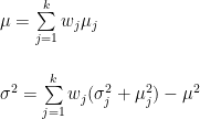
where 


Assuming that the Asian subpopulation variances 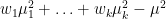
I do not have ethnically disaggregated SAT data for Asian-Americans, but Pang et al. (2011) reported means and SDs in the California Achievement Tests for several total cohorts of Asian seventh-grade students in California. This large and diverse sample can be used to probe the effects of ethnic heterogeneity on test score distributions. The tests were taken between 2003 and 2008 by consecutive cohorts, with 260,000 Asian students in total participating. The results were disaggregated by ethnicity, and look like this, with whites included for comparison:
| Reading | Math | |||||||
| Ethnicity | Mean | SD | Mean | SD | N | |||
|---|---|---|---|---|---|---|---|---|
| Asian Indian | 57.69 | 20.28 | 62.50 | 21.24 | 18816 | |||
The table shows several interesting things. There are some differences between the Asian groups: East Asians perform noticeably better, and some Southeast Asian groups noticeably worse, than whites, while the rest are roughly on par with whites. Asians are relatively better in math than in reading. Averaging over groups, whites have a tiny lead in the reading test, while Asians have a small advantage in the math test. Variability within the Asian groups in unremarkable: Asian-to-white variance ratios range from 0.81 to 1.06 in reading, and from 0.83 to 1.20 ín math. Compared to whites, overall variances in Asians, calculated using the normal mixture formulas given above, are 2 percent lower in reading and 8 percent higher in math. In the SAT, the Asian variance is about 28 percent (ERW) or 39 percent (math) higher than in whites (see Tables 3.5 and 3.7), while nothing like that is seen in the California Achievement Tests.
The mixing of several groups together does not increase the overall variance of Asians in the California tests much. This is so despite the fact that California has a large and ethnically highly heterogeneous Asian population, with substantial differences in mean test scores between subpopulations. The eleven states with high participation in the SAT that I analyzed in Chapter 3 probably each have a less diverse Asian population than California does. I therefore believe that ethnic heterogeneity explains little of the inflated Asian variances seen in the SAT.[Note 22]
Another possibility is that because the normality assumption is often violated in the SAT data, and the procedures for analyzing interval-censored data used in this post assume normality, the unusually large SAT variances estimated could be artefactual. To investigate this possibility, I used censored data methods to estimate the SDs (and means) of test score distributions for which the normality assumption is clearly violated, and for which SDs are also readily available in the College Board's reports. If censored data methods can recover SDs for such data with little bias, it suggests that the unusually large SDs seen in Asian SAT samples in particular are not due to a methodological artifact. The details of this investigation are reported in [Note 23], and they show that the methods used recover the true SDs with minimal bias. Therefore, it is unlikely that the unusually large SDs that I have found are artifacts of the estimation procedure. This does not mean that the normal distribution necessarily describes all aspects of the SAT distributions (e.g., the far right tail) accurately, but it does indicate that the high variability discussed above is a real phenomenon that warrants attention.
Yet another possible reason why the variance of Asian-American SAT scores is so large is assortative mating. Selective migration means that compared to Asians in Asia, the Asian-American population is above average in terms of heritable traits related to educational attainment. Consequently, the genotypes of Asian-American parents are correlated, leading to the expansion of phenotypic variance–this is because the variance of the sum of the additive effects of genotypes is larger if the genotypes are correlated. However, mating appears to be highly assortative in Asia to begin with, so it is difficult to say to what extent migration might increase assortativeness.
R code for analyzing distributional assumptions
# packages that may be used
# uncomment if you don't have these installed already

#install.packages("fitdistrplus")
#install.packages("ztable")
#install.packages("reshape2")
#install.packages("ggplot2")
#install.packages("ggrepel")
#install.packages("tigerstats")
#install.packages("sjPlot")
#install.packages("scales")
#install.packages("gridExtra")
#install.packahes("grid")

# read California Achievement Tests data
california_data <- read.csv(text="Ethnicity,reading_M,reading_SD,math_M,math_SD,N
Asian_Indian,57.69,20.28,62.5,21.24,18816
Cambodian,45.71,19.14,49.7,19.82,7009
Chinese,62.86,20.07,71.37,18.53,54330
Filipino,53.35,18.31,57.13,18.77,63860
Japanese,63.04,19.15,68.69,18.38,10905
Korean,61.2,19.23,70.76,17.88,21362
Lao,44.73,18.25,48.22,19,6763
Other_Asian,55.32,20.87,60.05,21.56,45748
Vietnamese,56.77,19.12,64.12,19,28737
White,58.15,20.29,57.72,19.66,752729")

# calculate overall mean and SD for Asians
california_data <- rbind(california_data, california_data[10,])
california_data[10,] <- with(california_data, list("All_Asians", round(weighted.mean(reading_M[1:9], N[1:9]),2), NA, round(weighted.mean(math_M[1:9], N[1:9]),2), NA, sum(N[1:9])))
california_data[10,3] <- round(sqrt(with(california_data, sum(sapply(1:9, function(i) N[i]/N[10]*(reading_SD[i]^2 + reading_M[i]^2)))-reading_M[10]^2)), 2)
california_data[10,5] <- round(sqrt(with(california_data, sum(sapply(1:9, function(i) N[i]/N[10]*(math_SD[i]^2 + math_M[i]^2)))-math_M[10]^2)), 2)

# html table of California Achievement Tests
cnames <- colnames(california_data)
california_data$Ethnicity<-gsub("_", " ", california_data$Ethnicity)
colnames(california_data) <- c("Ethnicity","Mean","SD","Mean","SD","N")
cgroup <- c("", "Reading", "Math", "")
n.cgroup <- c(1,2,2,1)

california_table <- ztable(california_data,zebra=2,zebra.color="#d4effc;", caption="Table 5.1. Summary data from California Achievement Tests, 2003--2008", caption.placement="top",caption.position="l", caption.bold=TRUE, align="lrrrrr",include.rownames=FALSE,size=5,colnames.bold=TRUE)
california_table  <- addcgroup(california_table, cgroup, n.cgroup)
california_table <- hlines(california_table, add = c(9))
capture.output(california_table,file="table5_1.html")
colnames(california_data) <- cnames
6. Racial and ethnic differences in other tests
Previously, I noted that the Asian advantage is currently larger in the SAT than in certain other tests of cognitive ability. To further explore this issue, and to generally compare the SAT to other tests, I will next examine three additional data sources: the National Assessment of Educational Progress (NAEP), the OECD's Programme for International Student Assessment (PISA), and the ACT test.
From 2005–2019, there were five NAEP main assessment studies of 12th grade students.[Note 24] The standardized NAEP math and reading gaps are shown in Figures 6.1 and 6.2. Because sample sizes for some groups are on the small side in the NAEP, I have displayed 95% confidence intervals for the d values in the graphs.
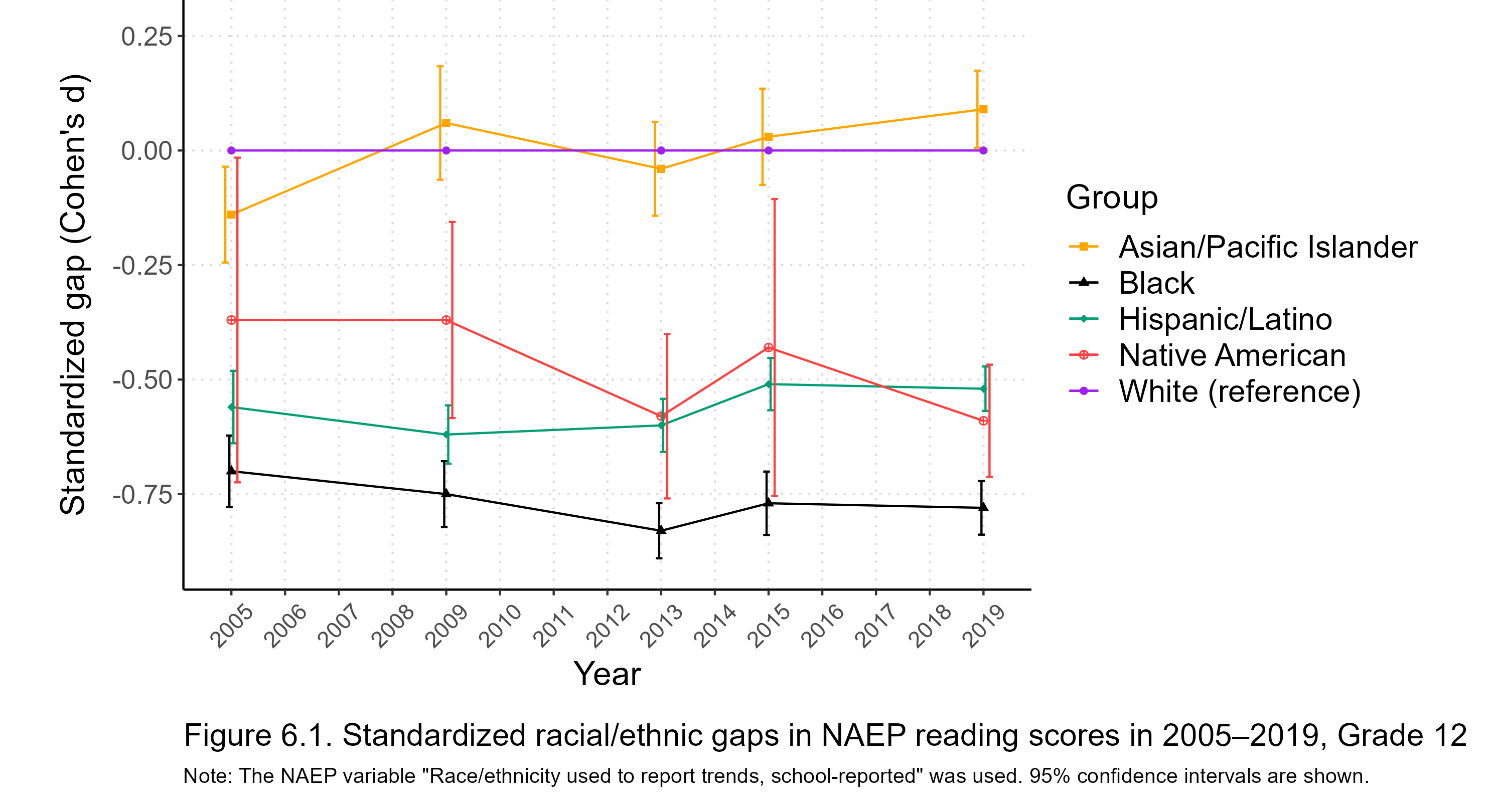
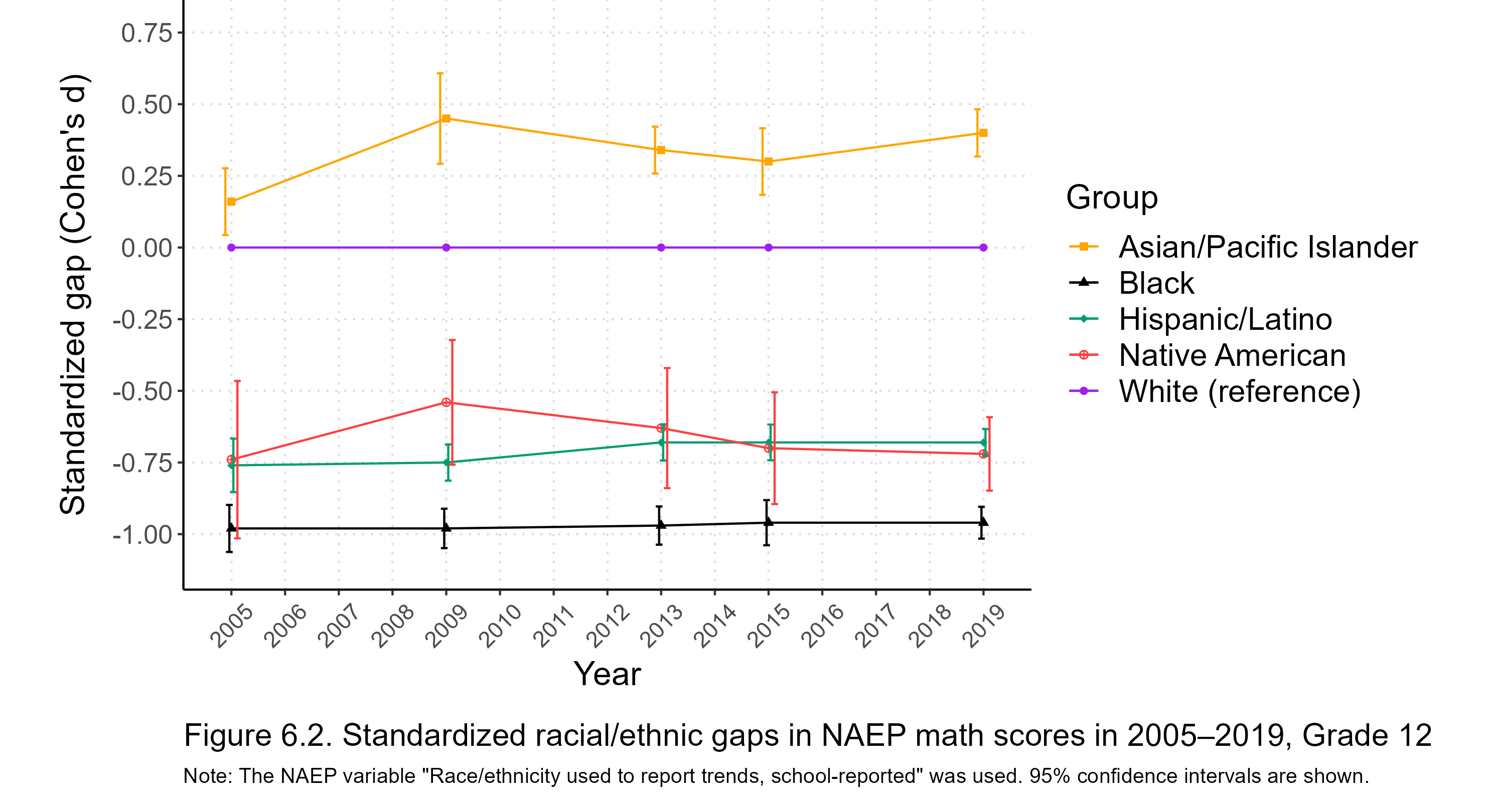
The NAEP time series overlap with my SAT data, enabling comparisons of the same high school senior cohorts in the two tests. In contrast to the SAT, the NAEP gaps are generally stable over the time period considered. In particular, the year 2017 is not a turning point of any kind in the NAEP results. Asians do not bolt away from whites nor can we say that Native American test performance collapses, although some decline in their scores may have happened over years. White-black and white-Hispanic gaps change slightly at best over 2005–2019 in the NAEP. The samples are not large enough to make conclusions about small changes, but major shifts of the kind seen in the national SAT data are not supported.
I do not know what the correlation of the NAEP reading and math scales is, but assuming a correlation of 0.75, the composite reading + math gaps in 2019 are 0.26 (Asian), -0.93 (black), and -0.64 (Hispanic). The composite d formula discussed in [Note 18] was used for these estimates. The corresponding SAT estimates in high-participation states, from Table 3.3, are 0.47 (Asian), -0.98 (black), and -0.71 (Hispanic).
Moving on to the next test, I retrieved PISA data from the International Data Explorer. Standardized gaps in the math, reading, and science tests among 15-year-old American students in 2000–2018 are shown in the next three figures.
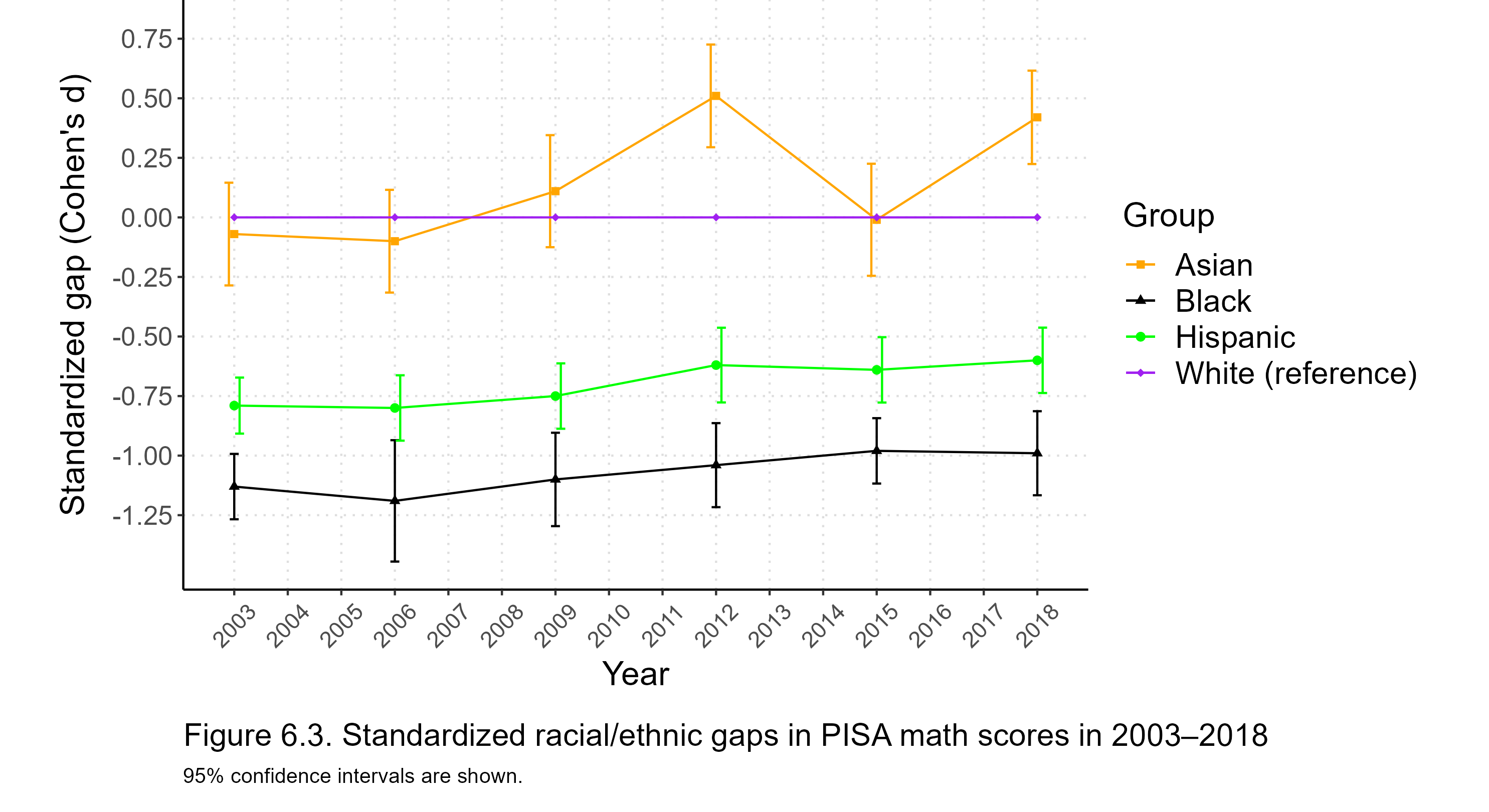
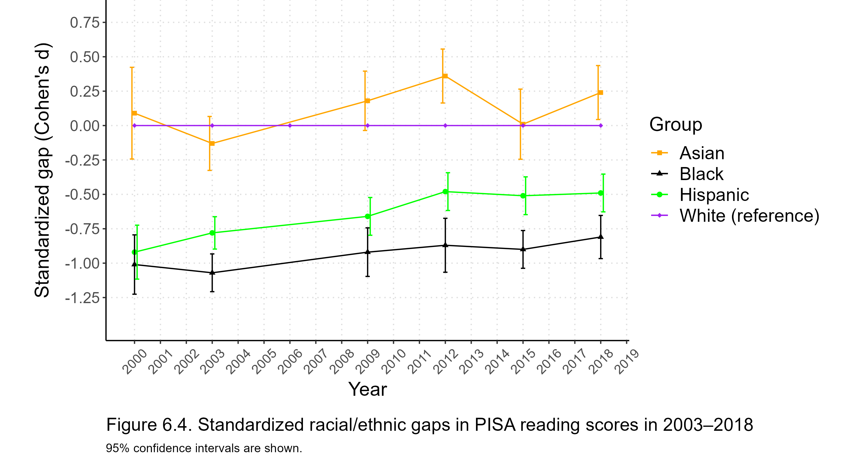
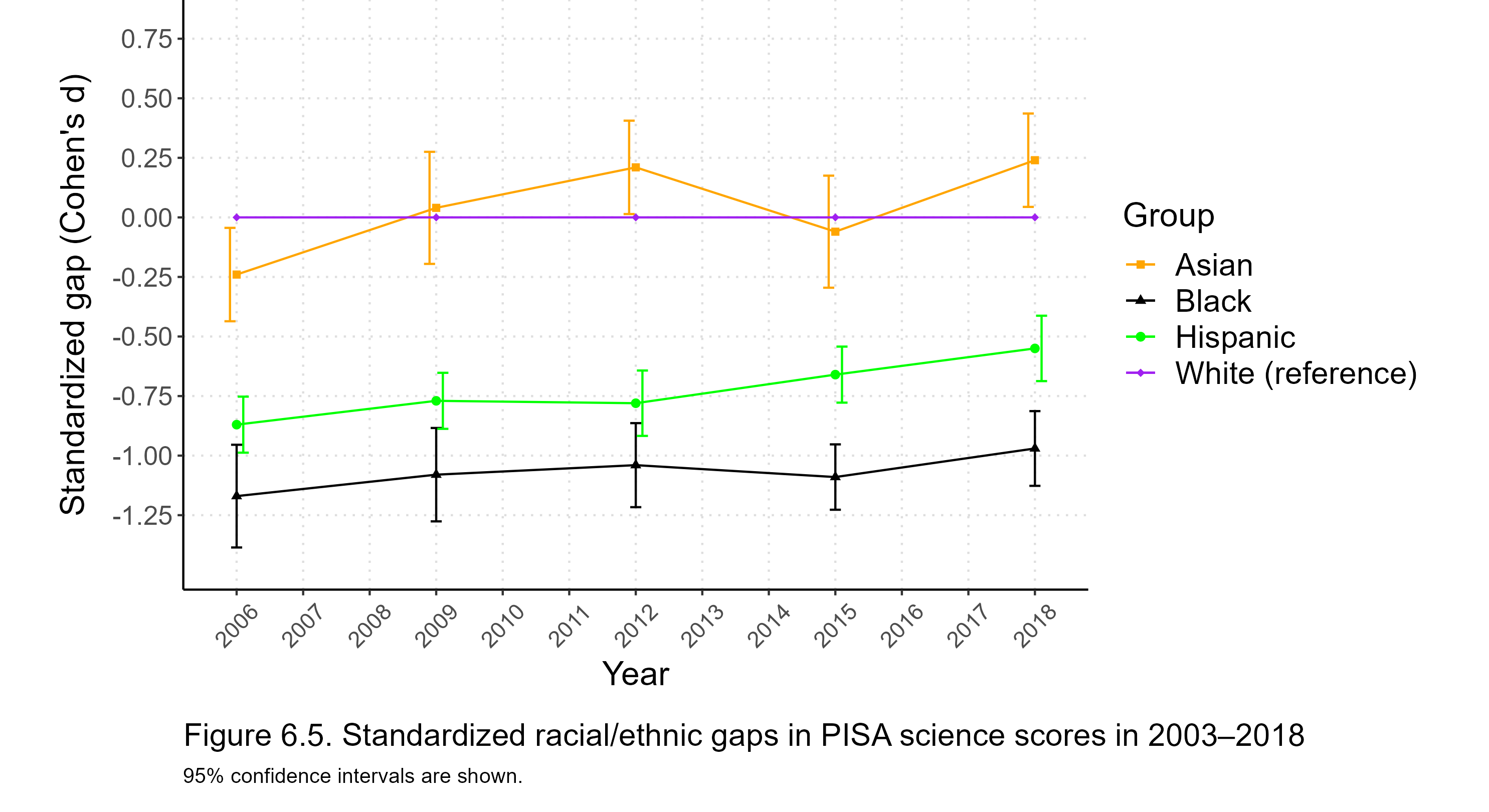
There is evidence of non-white groups gaining on whites in the PISA tests over time, but the math and reading gaps in the most recent assessments are quite similar to the NAEP math and reading gaps. The Asian-white gaps are smaller in the PISA than in the SAT, too. The intercorrelations of the three PISA tests are 0.80, on the average (see Table 2 in Taht et al., 2002), so the point estimates for the Asian-white, black-white, and Hispanic-white PISA composite score d values in 2018 come to 0.32, -0.99, and -0.59, respectively.
The SAT is a high-stakes test, while the NAEP or the PISA tests are not. Nevertheless, I do not think that the SAT necessarily provides better estimates of racial/ethnic differences in cognitive ability. For one thing, group differences in preparation for the SAT may result in somewhat biased estimates of ability gaps. In contrast, students do not generally prepare for a low-stakes test, so that will not be a source of bias in such tests, and while low motivation may be a concern in that setting, it is not expected to be correlated with race/ethnicity.
The NAEP and PISA results lend support to the argument that the current SAT version may somewhat overestimate the cognitive ability of Asian Americans. The post-2017 gains seen by Asians in the SAT are unlikely to be purely gains in ability. Without the test redesign, Asians would have grown their lead over whites and others at a slower rate, given the test score gap trends seen during the previous SAT versions. The long-term improvement in Asian-American test performance is almost certainly a reflection of Asian immigration to America becoming more educationally selective in recent generations. Fundamentally, it is about improvements in the education-related genetic characteristics of the Asian-American population.
One open question with respect to Asian Americans is how being a foreign-born, non-native speaker of English affects SAT scores. This cannot be analyzed with any specificity based on the data the College Board makes public. A previous analysis on this blog suggests that nativity may have a big effect on Asian test performance, but besides the analytical limitations mentioned in that post, the data used there are from the year 2000 at the latest, whereas the Asian American population has roughly doubled in size in the 21st century so far. This is almost entirely due to high levels of immigration. Therefore, Asian American test performance in the 20th century or even the aughts is not necessarily a good guide to the current situation. The trend is for Asians to pull further away from everyone else in the SAT and other tests, and if a larger share of them are native-born in the future, this tendency may even accelerate.
The NAEP and PISA tests can also be used to investigate whether there are differences in the variability of test scores between racial/ethnic groups. Figures 6.6a through 6.6e make this comparison.
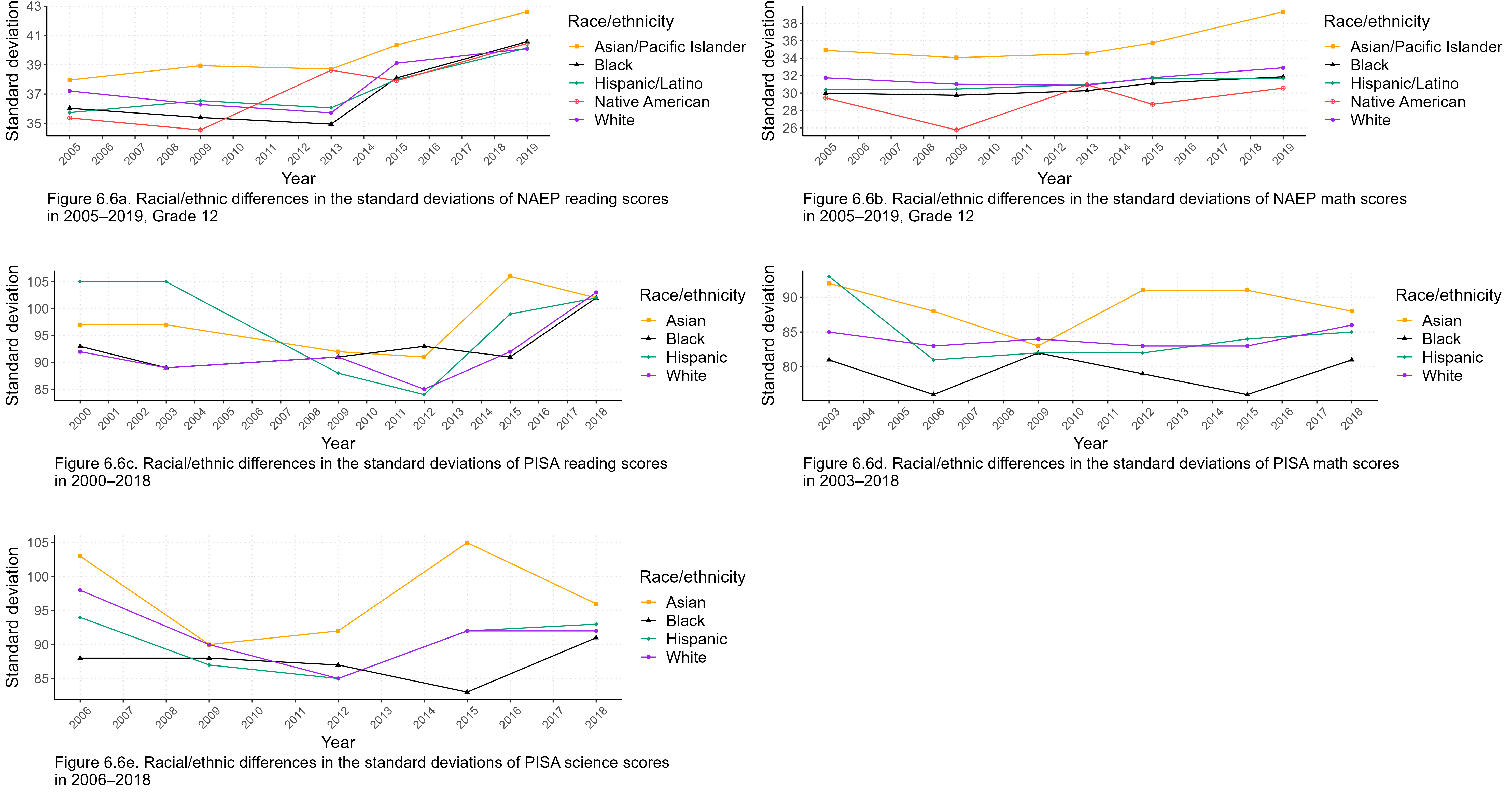
The figures indicate that Asian SDs are substantially and rather consistently larger than those of other groups in the NAEP and PISA tests. Therefore, the greater variability of Asians is not something that is seen only in the SAT. On the other hand, in the California Achievement Tests analyzed in Chapter 5 there was little evidence of excess Asian variability, so the generality of this phenomenon is unclear.
The ACT was introduced in 1959 as a competitor to the SAT which had debuted in 1926. Traditionally, the ACT is the preferred test in "flyover states", and the SAT on the East and West coasts. The ACT is currently somewhat less popular nationally than the SAT. Some students take both tests, but strong regional biases towards one or the other remain. All colleges that consider test scores in admissions accept both tests.
The ACT has four main sections assessing skills in English, math, reading, and scientific reasoning. The ACT composite score has a range from 1 to 36 (with individual scores rounded to integers), and has historically had a mean of about 20 to 21 in the total national cohort, with a pooled SD of about 5 to 6. The following figure shows ACT composite scores by race/ethnicity nationally from 2002 through 2022. The data were obtained from the Digest of Education Statistics (here and here), and, for the most recent year, from this report.

National test score trends in the ACT seem rather similar to the SAT, except that the ACT has preserved the meaning of its scale points better over years (cf., Figure 1.1 in Chapter 1). Asians seem to be pulling away from everyone else over the last half dozen years in the ACT, too, and Native American performance is on a long-term decline in this test as well. Participation in the ACT has decreased precipitously in recent years, from over 2 million test-takers in 2016 and 2017 to only 1.3 million in 2022.
Unfortunately, within-group SDs are not available for the ACT, so standardized racial/ethnic differences cannot be properly calculated. The next figure uses the pooled national SDs to estimate the gaps, so the estimates are biased to some degree, probably towards zero, due to this limitation. The pooled SDs are available for all years with the exception of 2019, which is skipped in the figure.

Interpretation of the trends in Figures 6.7 and 6.8 is made hard by changes in the composition of the test-taking cohorts. In addition to large fluctuations in the total number of test-takers, selection into participation has been much influenced by policies adopted in many states over the last ten years or so whereby all high school juniors or seniors are expected to take the ACT. Those states tend to be whiter and less Asian than average, which skews the composition of the national ACT cohorts.
I looked at ACT results in states where high-schoolers universally take the test, but it appears that at least in light of SEDA test data from the same states, the ACT states are less representative of the American population and specific racial/ethnic groups in terms of cognitive ability than the high SAT-participation states. This means that using ACT data to estimate ability gaps in the general population would be a lot more challenging than using SAT data for this purpose, so state-level ACT results are discussed only in a footnote.[Note 25]
NAEP results by race/ethnicity in 2005–2019
Year,Group,Reading_Mean,Reading_SE,Reading_SD,Reading_N,Reading_d,Reading_d_SE,Math_Mean,Math_SE,Math_SD,Math_N,Math_d,Math_d_SE
2005,Asian/Pacific Islander,287.48,1.88,37.96,408,-0.14,0.0533843625266421,162.62,1.98,34.9,311,0.16,0.0594155376866495
2005,Black,266.69,1.2,36.03,902,-0.7,0.0396949280816186,126.62,1.09,29.98,757,-0.98,0.0418703998693989
2005,Hispanic/Latino,271.95,1.23,35.74,844,-0.56,0.0403352443080105,133.47,1.32,30.4,530,-0.76,0.0476981047884575
2005,Native American,278.82,6.32,35.37,31,-0.37,0.180777221431015,134.16,4.07,29.44,52,-0.74,0.140092086866394
2005,Two or more races,283.17,6.1,34.05,31,-0.26,0.180739737611703,142.2,3.57,36.1,102,-0.48,0.10074632476621
2005,White (reference),292.69,0.74,37.21,2528,0,0.0281271975231506,157.48,0.56,31.75,3214,0,0.0249454912916334
2009,Asian/Pacific Islander,298.26,2.37,38.94,270,0.06,0.0631406542052497,175.19,2.67,34.07,163,0.45,0.0806535789509241
2009,Black,268.95,1.12,35.4,999,-0.75,0.0366820210154704,131.01,0.83,29.75,1285,-0.98,0.0350562570604821
2009,Hispanic/Latino,273.57,0.99,36.55,1363,-0.62,0.0324879347089682,138.01,0.77,30.46,1565,-0.75,0.03222952148381
2009,Native American,282.52,3.73,34.55,86,-0.37,0.109221636390022,144.49,2.81,25.76,84,-0.54,0.110861486239393
2009,Two or more races,298.29,3.24,35.32,119,0.06,0.0932009623470645,157.74,3.03,32.12,112,-0.11,0.0962712342954692
2009,White (reference),295.98,0.61,36.29,3539,0,0.0237724923608965,161.11,0.57,31.02,2962,0,0.0259849850167371
2013,Asian/Pacific Islander,296.01,1.92,38.71,406,-0.04,0.0523077632071865,172.14,1.27,34.54,740,0.34,0.041626862418014
2013,Black,267.7,0.86,34.95,1652,-0.83,0.0307080660760922,131.82,0.79,30.27,1468,-0.97,0.0340272654329969
2013,Hispanic/Latino,275.65,0.86,36.06,1758,-0.6,0.0295784332882785,140.52,0.77,30.98,1619,-0.68,0.032179922902083
2013,Native American,276.66,3.47,38.63,124,-0.58,0.0915520755055838,141.95,3.25,30.95,91,-0.63,0.10688295008002
2013,Two or more races,290.95,2.51,37.03,218,-0.18,0.0697436838807522,155.12,1.68,31.94,361,-0.21,0.0560537809572586
2013,White (reference),297.29,0.59,35.72,3665,0,0.0233602780824054,161.52,0.59,30.89,2741,0,0.0270122325580631
2015,Asian/Pacific Islander,296.72,2.05,40.34,387,0.03,0.0535622438952258,170,2,35.75,320,0.3,0.0592344829030099
2015,Black,265.64,1.14,38.1,1117,-0.77,0.0352726201037202,129.87,1.04,31.13,896,-0.96,0.0401592016094045
2015,Hispanic/Latino,275.71,0.88,37.99,1864,-0.51,0.0290775546023106,138.66,0.77,31.69,1694,-0.68,0.0318071690218829
2015,Native American,278.62,6.23,37.91,37,-0.43,0.165341821076456,138.09,2.79,28.71,106,-0.7,0.0994477932810513
2015,Two or more races,295.05,2.91,40.32,192,-0.01,0.0741158956165392,157.26,2.19,33.76,238,-0.09,0.0676159931357712
2015,White (reference),295.5,0.66,39.11,3511,0,0.0238670961721864,160.18,0.61,31.76,2711,0,0.0271612804020732
2019,Asian/Pacific Islander,298.51,1.7,42.62,629,0.09,0.0429584312780394,172.96,1.51,39.34,679,0.4,0.0419550308717296
2019,Black,263.48,0.98,40.58,1715,-0.78,0.0298621548001836,128.35,0.68,31.87,2197,-0.96,0.0283266721433815
2019,Hispanic/Latino,273.96,0.74,40.15,2944,-0.52,0.0247804678375332,137.54,0.52,31.71,3719,-0.68,0.0238590417389412
2019,Native American,271.51,2.43,40.46,277,-0.59,0.0625000087220008,136,1.92,30.57,254,-0.72,0.0653575923427061
2019,Two or more races,295.11,2.12,41.54,384,0,0.0534684845671601,156.77,1.88,35.4,355,-0.08,0.0555602349714816
2019,White (reference),295,0.64,40.1,3926,0,0.0225704308883094,159.44,0.54,32.91,3714,0,0.0232056665874154
PISA results by race/ethnicity in 2000–2018
Year,Test,White_Mean,White_SE,White_SD,Black_Mean,Black_SE,Black_SD,Hispanic_Mean,Hispanic_SE,Hispanic_SD,Asian_Mean,Asian_SE,Asian_SD,Other_Mean,Other_SE,Other_SD,Multiracial_Mean,Multiracial_SE,Multiracial_SD,White_N,Black_N,Hispanic_N,Asian_N,Other_N,Multiracial_N
2018,Math,503,3.4,86,419,5.8,81,452,4.6,85,539,7.9,88,474,5.8,89,NA,NA,NA,640,195,341,124,235,NA
2015,Math,499,2.8,83,419,4.7,76,446,5.2,84,498,10.1,91,423,16.4,83,475,7,82,879,261,261,81,26,137
2012,Math,506,3.7,83,421,6.2,79,455,4.8,82,549,9,91,436,8.7,69,492,7.4,84,503,162,292,102,63,129
2009,Math,515,3.9,84,423,6.6,82,453,3.8,82,524,9.6,83,460,21.1,76,487,6.4,87,464,154,466,75,13,185
2006,Math,502,3.1,83,404,8.9,76,436,4.5,81,494,8.7,88,446,9.6,71,482,7.6,80,717,73,324,102,55,111
2003,Math,512,2.5,85,417,5.1,81,443,5.1,93,506,9.8,92,446,26.5,111,502,6.4,86,1156,252,333,88,18,181
2018,Reading,531,3.8,103,448,7.1,102,481,5.7,102,556,9,102,501,5.7,103,NA,NA,NA,735,206,320,128,327,NA
2015,Reading,526,3.3,92,443,5.4,91,478,5.7,99,527,13.3,106,440,14.8,99,498,7.1,94,777,284,302,64,45,175
2012,Reading,519,4.1,85,443,8.3,93,478,4.5,84,550,8.1,91,438,9.5,81,517,7.6,86,430,126,348,126,73,128
2009,Reading,525,3.8,91,441,7.2,91,466,4.3,88,541,9.4,92,462,28.6,88,502,6.4,93,573,160,419,96,9,211
2003,Reading,525,2.6,89,430,5.6,89,453,5.9,105,513,9.2,97,456,26.8,114,515,7.3,93,1172,253,317,111,18,162
2000,Reading,538,5.1,92,445,8.2,93,449,7.6,105,546,15.8,97,455,14,96,NA,NA,NA,325,129,191,38,47,NA
2018,Science,529,3.4,92,440,6.3,91,478,5.1,93,551,9.4,96,502,6.1,95,NA,NA,NA,732,209,333,104,243,NA
2015,Science,531,2.8,92,433,4.9,83,470,4.8,92,525,12,105,462,11.5,87,503,6.4,92,1080,287,367,77,57,207
2012,Science,528,3.7,85,439,6.8,87,462,4.7,85,546,8.6,92,439,10.3,78,511,7.8,89,528,164,327,114,57,130
2009,Science,532,4,90,435,7.2,88,464,3.8,87,536,9.7,90,465,31.3,93,503,7.6,96,506,149,524,86,9,160
2006,Science,523,3,98,409,8.8,88,439,4.7,94,499,9.7,103,453,12.1,87,501,8,94,1067,100,400,113,52,138
National ACT results by race/ethnicity in 2002–2022
Year,Group,Composite_Mean,Composite_SD,N
2002,All groups,20.8,4.8,1116082
2002,White,21.7,NA,NA
2002,Black,16.8,NA,NA
2002,Hispanic,18.4,NA,NA
2002,Asian/Pacific Islander,21.6,NA,NA
2002,Native American,18.6,NA,NA
2002,Asian,NA,NA,NA
2002,Pacific Islander,NA,NA,NA
2002,Two or more races,NA,NA,NA
2003,All groups,20.8,4.8,1175059
2003,White,21.7,NA,NA
2003,Black,16.9,NA,NA
2003,Hispanic,18.5,NA,NA
2003,Asian/Pacific Islander,21.8,NA,NA
2003,Native American,18.7,NA,NA
2003,Asian,NA,NA,NA
2003,Pacific Islander,NA,NA,NA
2003,Two or more races,NA,NA,NA
2004,All groups,20.9,4.8,1171460
2004,White,21.8,NA,NA
2004,Black,17.1,NA,NA
2004,Hispanic,18.5,NA,NA
2004,Asian/Pacific Islander,21.9,NA,NA
2004,Native American,18.8,NA,NA
2004,Asian,NA,NA,NA
2004,Pacific Islander,NA,NA,NA
2004,Two or more races,NA,NA,NA
2005,All groups,20.9,4.8,1186000
2005,White,21.9,NA,NA
2005,Black,17,NA,NA
2005,Hispanic,18.6,NA,NA
2005,Asian/Pacific Islander,22.1,NA,NA
2005,Native American,18.7,NA,NA
2005,Asian,NA,NA,NA
2005,Pacific Islander,NA,NA,NA
2005,Two or more races,NA,NA,NA
2006,All groups,21.1,4.8,1206000
2006,White,22,NA,NA
2006,Black,17.1,NA,NA
2006,Hispanic,18.6,NA,NA
2006,Asian/Pacific Islander,22.3,NA,NA
2006,Native American,18.8,NA,NA
2006,Asian,NA,NA,NA
2006,Pacific Islander,NA,NA,NA
2006,Two or more races,NA,NA,NA
2007,All groups,21.2,5,1300599
2007,White,22.1,NA,NA
2007,Black,17,NA,NA
2007,Hispanic,18.7,NA,NA
2007,Asian/Pacific Islander,22.6,NA,NA
2007,Native American,18.9,NA,NA
2007,Asian,NA,NA,NA
2007,Pacific Islander,NA,NA,NA
2007,Two or more races,NA,NA,NA
2008,All groups,21.1,5,1421941
2008,White,22.1,NA,NA
2008,Black,16.9,NA,NA
2008,Hispanic,18.7,NA,NA
2008,Asian/Pacific Islander,22.9,NA,NA
2008,Native American,19,NA,NA
2008,Asian,NA,NA,NA
2008,Pacific Islander,NA,NA,NA
2008,Two or more races,NA,NA,NA
2009,All groups,21.1,5.1,1480469
2009,White,22.2,NA,NA
2009,Black,16.9,NA,NA
2009,Hispanic,18.7,NA,NA
2009,Asian/Pacific Islander,23.2,NA,NA
2009,Native American,18.9,NA,NA
2009,Asian,NA,NA,NA
2009,Pacific Islander,NA,NA,NA
2009,Two or more races,NA,NA,NA
2010,All groups,21,5.2,1568835
2010,White,22.3,NA,NA
2010,Black,16.9,NA,NA
2010,Hispanic,18.6,NA,NA
2010,Asian/Pacific Islander,23.4,NA,NA
2010,Native American,19,NA,NA
2010,Asian,NA,NA,NA
2010,Pacific Islander,NA,NA,NA
2010,Two or more races,NA,NA,NA
2011,All groups,21.1,5.2,1623112
2011,White,22.4,NA,NA
2011,Black,17,NA,NA
2011,Hispanic,18.7,NA,NA
2011,Asian/Pacific Islander,NA,NA,NA
2011,Native American,18.6,NA,NA
2011,Asian,23.6,NA,NA
2011,Pacific Islander,19.5,NA,NA
2011,Two or more races,21.1,NA,NA
2012,All groups,21.1,5.3,1666017
2012,White,22.4,NA,NA
2012,Black,17,NA,NA
2012,Hispanic,18.9,NA,NA
2012,Asian/Pacific Islander,NA,NA,NA
2012,Native American,18.4,NA,NA
2012,Asian,23.6,NA,NA
2012,Pacific Islander,19.8,NA,NA
2012,Two or more races,21.4,NA,NA
2013,All groups,20.9,5.4,1799243
2013,White,22.2,NA,NA
2013,Black,16.9,NA,NA
2013,Hispanic,18.8,NA,NA
2013,Asian/Pacific Islander,NA,NA,NA
2013,Native American,18,NA,NA
2013,Asian,23.5,NA,NA
2013,Pacific Islander,19.5,NA,NA
2013,Two or more races,21.1,NA,NA
2014,All groups,21,5.4,1845787
2014,White,22.3,NA,NA
2014,Black,17,NA,NA
2014,Hispanic,18.8,NA,NA
2014,Asian/Pacific Islander,NA,NA,NA
2014,Native American,18,NA,NA
2014,Asian,23.5,NA,NA
2014,Pacific Islander,18.6,NA,NA
2014,Two or more races,21.2,NA,NA
2015,All groups,21,5.5,1924436
2015,White,22.4,NA,NA
2015,Black,17.1,NA,NA
2015,Hispanic,18.9,NA,NA
2015,Asian/Pacific Islander,NA,NA,NA
2015,Native American,17.9,NA,NA
2015,Asian,23.9,NA,NA
2015,Pacific Islander,18.8,NA,NA
2015,Two or more races,21.2,NA,NA
2016,All groups,20.8,5.6,2090342
2016,White,22.2,NA,NA
2016,Black,17,NA,NA
2016,Hispanic,18.7,NA,NA
2016,Asian/Pacific Islander,NA,NA,NA
2016,Native American,17.7,NA,NA
2016,Asian,24,NA,NA
2016,Pacific Islander,18.6,NA,NA
2016,Two or more races,21,NA,NA
2017,All groups,21,5.6,2030038
2017,White,22.4,NA,NA
2017,Black,17.1,NA,NA
2017,Hispanic,18.9,NA,NA
2017,Asian/Pacific Islander,NA,NA,NA
2017,Native American,17.5,NA,NA
2017,Asian,24.3,NA,NA
2017,Pacific Islander,18.4,NA,NA
2017,Two or more races,21.2,NA,NA
2018,All groups,20.8,5.8,1914817
2018,White,22.2,NA,NA
2018,Black,16.9,NA,NA
2018,Hispanic,18.8,NA,NA
2018,Asian/Pacific Islander,NA,NA,NA
2018,Native American,17.3,NA,NA
2018,Asian,24.5,NA,NA
2018,Pacific Islander,18.2,NA,NA
2018,Two or more races,21.1,NA,NA
2019,All groups,20.7,NA,1782820
2019,White,22.1,NA,NA
2019,Black,16.8,NA,NA
2019,Hispanic,18.7,NA,NA
2019,Asian/Pacific Islander,NA,NA,NA
2019,Native American,17,NA,NA
2019,Asian,24.6,NA,NA
2019,Pacific Islander,17.9,NA,NA
2019,Two or more races,21,NA,NA
2020,All groups,20.6,6,1670497
2020,White,22,NA,NA
2020,Black,16.7,NA,NA
2020,Hispanic,18.5,NA,NA
2020,Asian/Pacific Islander,NA,NA,NA
2020,Native American,16.7,NA,NA
2020,Asian,24.9,NA,NA
2020,Pacific Islander,17.5,NA,NA
2020,Two or more races,20.9,NA,NA
2021,All groups,20.3,6,1295349
2021,White,21.7,NA,NA
2021,Black,16.3,NA,NA
2021,Hispanic,18.3,NA,NA
2021,Asian/Pacific Islander,NA,NA,NA
2021,Native American,16.9,NA,NA
2021,Asian,24.9,NA,NA
2021,Pacific Islander,17.2,NA,NA
2021,Two or more races,20.6,NA,NA
2022,All groups,19.8,5.9,1349644
2022,White,21.3,NA,708952
2022,Asian,24.7,NA,54464
2022,Black,16.1,NA,153579
2022,Hispanic,17.7,NA,210205
2022,Native American,16.4,NA,10728
2022,Pacific Islander,17.1,NA,2961
2022,Two or more races,20.1,NA,64330
2022,No response,17.6,NA,144425
R code for NAEP, PISA, and ACT analyses
# calculate standardized 12th grade reading gaps in the NAEP data

# read NAEP reading data
naep_reading <- read.csv(text="Year,Group,Reading_Mean,Reading_SE,Reading_SD
2019,White,295,0.64,40.1
2019,Black,263.48,0.98,40.58
2019,Hispanic/Latino,273.96,0.74,40.15
2019,Asian/Pacific Islander,298.51,1.7,42.62
2019,Native American,271.51,2.43,40.46
2019,Two or more races,295.11,2.12,41.54
2015,White,295.5,0.66,39.11
2015,Black,265.64,1.14,38.1
2015,Hispanic/Latino,275.71,0.88,37.99
2015,Asian/Pacific Islander,296.72,2.05,40.34
2015,Native American,278.62,6.23,37.91
2015,Two or more races,295.05,2.91,40.32
2013,White,297.29,0.59,35.72
2013,Black,267.7,0.86,34.95
2013,Hispanic/Latino,275.65,0.86,36.06
2013,Asian/Pacific Islander,296.01,1.92,38.71
2013,Native American,276.66,3.47,38.63
2013,Two or more races,290.95,2.51,37.03
2009,White,295.98,0.61,36.29
2009,Black,268.95,1.12,35.4
2009,Hispanic/Latino,273.57,0.99,36.55
2009,Asian/Pacific Islander,298.26,2.37,38.94
2009,Native American,282.52,3.73,34.55
2009,Two or more races,298.29,3.24,35.32
2005,White,292.69,0.74,37.21
2005,Black,266.69,1.2,36.03
2005,Hispanic/Latino,271.95,1.23,35.74
2005,Asian/Pacific Islander,287.48,1.88,37.96
2005,Native American,278.82,6.32,35.37
2005,Two or more races,283.17,6.1,34.05")

# estimate Ns from standard errors and SDs
naep_reading$N <- with(naep_reading, round((Reading_SD/Reading_SE)^2,0))

# function for calculating gaps
cohen_d <- function(group1_mean, group1_sd, group1_N, group2_mean, group2_sd, group2_N)  {
s <- sqrt( ( (group1_N-1)*group1_sd^2 + (group2_N-1)*group2_sd^2 ) / (group1_N+group2_N-2) )
return (round(((group1_mean-group2_mean)/s),2))
}

# calculate d values
naep_reading$d <- sapply(1:nrow(naep_reading), function(i) with(naep_reading, cohen_d(Reading_Mean[i], Reading_SD[i], N[i], naep_reading[naep_reading$Group == "White" & naep_reading$Year == Year[i],]$Reading_Mean, naep_reading[naep_reading$Group == "White" & naep_reading$Year == Year[i],]$Reading_SD,
naep_reading[naep_reading$Group == "White" & naep_reading$Year == Year[i],]$N)))

# function for calculating standard errors for Cohen's d
cohen_d_se <- function(n1, n2, d) {
variance <- ( ( (n1 + n2) / (n1 * n2) ) + ( d^2 / (2*(n1 + n2 - 2)) ) )
return(sqrt(variance))
}

naep_reading$d_SE <- sapply(1:nrow(naep_reading), function(i) with(naep_reading, cohen_d_se(N[i], naep_reading[naep_reading$Group=="White" & naep_reading$Year==Year[i],]$N, d[i])))

naep_reading[naep_reading$Group=="White",]$Group <- "White (reference)"

# graph of standardized national NAEP reading score gaps
library(ggplot2)
ggplot(data=subset(naep_reading, !(Group %in% c("White (reference)", "Two or more races"))), aes(Year, d, color=Group, shape=Group)) +
geom_point(position=position_dodge())+
geom_line(linetype = "solid",position=position_dodge())+
theme_classic()+
theme(plot.margin = unit(c(0,0.4,0.4,0.4), "in"),plot.tag = element_text(size = 10), plot.tag.position =  c(0.523,-0.031), panel.grid.major = element_line(color = "gray87", linetype = "dotted"), text=element_text(size=16), plot.caption = element_text(hjust = 0, margin = margin(t = 15), size = 15), axis.text.x = element_text(size=11, vjust=0.5,angle=45), axis.title.y = element_text(margin = margin(r = 10)), legend.title=element_text(size=16), legend.text=element_text(size=15), axis.title.x = element_text(margin = margin(t = 5)))+
scale_y_continuous(breaks=c(-0.75, -0.50, -0.25, 0.00, 0.25),limits=c(-0.90,0.27))+
scale_x_continuous(breaks=c(2002:2022))+
scale_shape_manual(values=c(15,17,18,10,16))+
scale_color_manual(values=c("orange", "black", "#009E73", "brown1", "purple"))+
labs(tag = "Note: The NAEP variable \"Race/ethnicity used to report trends, school-reported\" was used. 95% confidence intervals are shown.", caption="Figure 6.1. Standardized racial/ethnic gaps in NAEP reading scores in 2005–2019, Grade 12",y="Standardized gap (Cohen's d)")+
geom_errorbar(aes(ymin = d-1.96*d_SE, ymax = d+1.96*d_SE), width=0.5,position=position_dodge(width=0.3))+
geom_point(data=subset(naep_reading, Group == "White (reference)"), aes(Year, d, color=Group, shape=Group))+
geom_line(data=subset(naep_reading, Group == "White (reference)"), aes(Year, d, color=Group, shape=Group), linetype = "solid")
ggsave("fig6_1.png", height=5.4, width=9.9, dpi=300)

# calculate standardized 12th grade math gaps in the NAEP data

# read NAEP math data
naep_math <- read.csv(text="Year,Group,Math_Mean,Math_SE,Math_SD
2019,White,159.44,0.54,32.91
2019,Black,128.35,0.68,31.87
2019,Hispanic/Latino,137.54,0.52,31.71
2019,Asian/Pacific Islander,172.96,1.51,39.34
2019,Native American,136,1.92,30.57
2019,Two or more races,156.77,1.88,35.4
2015,White,160.18,0.61,31.76
2015,Black,129.87,1.04,31.13
2015,Hispanic/Latino,138.66,0.77,31.69
2015,Asian/Pacific Islander,170,2,35.75
2015,Native American,138.09,2.79,28.71
2015,Two or more races,157.26,2.19,33.76
2013,White,161.52,0.59,30.89
2013,Black,131.82,0.79,30.27
2013,Hispanic/Latino,140.52,0.77,30.98
2013,Asian/Pacific Islander,172.14,1.27,34.54
2013,Native American,141.95,3.25,30.95
2013,Two or more races,155.12,1.68,31.94
2009,White,161.11,0.57,31.02
2009,Black,131.01,0.83,29.75
2009,Hispanic/Latino,138.01,0.77,30.46
2009,Asian/Pacific Islander,175.19,2.67,34.07
2009,Native American,144.49,2.81,25.76
2009,Two or more races,157.74,3.03,32.12
2005,White,157.48,0.56,31.75
2005,Black,126.62,1.09,29.98
2005,Hispanic/Latino,133.47,1.32,30.4
2005,Asian/Pacific Islander,162.62,1.98,34.9
2005,Native American,134.16,4.07,29.44
2005,Two or more races,142.2,3.57,36.1")

# estimate Ns from standard errors and SDs
naep_math$N <- with(naep_math, round((Math_SD/Math_SE)^2,0))

# calculate d values
naep_math$d <- sapply(1:nrow(naep_math), function(i) with(naep_math, cohen_d(Math_Mean[i], Math_SD[i], N[i], naep_math[naep_math$Group == "White" & naep_math$Year == Year[i],]$Math_Mean, naep_math[naep_math$Group == "White" & naep_math$Year == Year[i],]$Math_SD,
naep_math[naep_math$Group == "White" & naep_math$Year == Year[i],]$N)))

# function for calculating standard errors for Cohen's d
cohen_d_se <- function(n1, n2, d) {
variance <- ( ( (n1 + n2) / (n1 * n2) ) + ( d^2 / (2*(n1 + n2 - 2)) ) )
return(sqrt(variance))
}

naep_math$d_SE <- sapply(1:nrow(naep_math), function(i) with(naep_math, cohen_d_se(N[i], naep_math[naep_math$Group=="White" & naep_math$Year==Year[i],]$N, d[i])))

naep_math[naep_math$Group=="White",]$Group <- "White (reference)"

# graph of standardized NAEP national math score gaps
ggplot(data=subset(naep_math, !(Group %in% c("White (reference)", "Two or more races"))), aes(Year, d, color=Group, shape=Group)) +
geom_point(position=position_dodge())+
geom_line(linetype = "solid",position=position_dodge())+
theme_classic()+
theme(plot.margin = unit(c(0,0.4,0.4,0.4), "in"),plot.tag = element_text(size = 10), plot.tag.position =  c(0.523,-0.031), panel.grid.major = element_line(color = "gray87", linetype = "dotted"), text=element_text(size=16), plot.caption = element_text(hjust = 0, margin = margin(t = 15), size = 15), axis.text.x = element_text(size=11, vjust=0.5,angle=45), axis.title.y = element_text(margin = margin(r = 10)), legend.title=element_text(size=16), legend.text=element_text(size=15), axis.title.x = element_text(margin = margin(t = 5)))+
scale_y_continuous(breaks=c(-1.00, -0.75, -0.50, -0.25, 0.00, 0.25, 0.50, 0.75),limits=c(-1.1,0.77))+
scale_x_continuous(breaks=c(2002:2022))+
scale_shape_manual(values=c(15,17,18,10,16))+
scale_color_manual(values=c("orange", "black", "#009E73", "brown1", "purple"))+
labs(tag = "Note: The NAEP variable \"Race/ethnicity used to report trends, school-reported\" was used. 95% confidence intervals are shown.", caption="Figure 6.2. Standardized racial/ethnic gaps in NAEP math scores in 2005–2019, Grade 12",y="Standardized gap (Cohen's d)")+
geom_errorbar(aes(ymin = d-1.96*d_SE, ymax = d+1.96*d_SE), width=0.5,position=position_dodge(width=0.3))+
geom_point(data=subset(naep_math, Group == "White (reference)"), aes(Year, d, color=Group, shape=Group))+
geom_line(data=subset(naep_math, Group == "White (reference)"), aes(Year, d, color=Group, shape=Group), linetype = "solid")
ggsave("fig6_2.png", height=5.4, width=9.9, dpi=300)

# combine all standardized NAEP gaps into one table
naep_table <- naep_reading
colnames(naep_table) <- c(colnames(naep_table)[1:5], "Reading_N", "Reading_d", "Reading_d_SE")
naep_table <- merge(naep_table,naep_math,all=TRUE)
colnames(naep_table) <- c(colnames(naep_table)[1:11], "Math_N", "Math_d", "Math_d_SE")

# estimate composite gaps

r <- 0.75 # assumed correlation
# Asian
sum((naep_reading[naep_reading$Year==2019 & naep_reading$Group=="Asian/Pacific Islander",]$d + naep_math[naep_math$Year==2019 & naep_math$Group=="Asian/Pacific Islander",]$d) / sqrt(2 + 2*r))
# black
sum((naep_reading[naep_reading$Year==2019 & naep_reading$Group=="Black",]$d + naep_math[naep_math$Year==2019 & naep_math$Group=="Black",]$d) / sqrt(2 + 2*r))
# Hispanic
sum((naep_reading[naep_reading$Year==2019 & naep_reading$Group=="Hispanic/Latino",]$d + naep_math[naep_math$Year==2019 & naep_math$Group=="Hispanic/Latino",]$d) / sqrt(2 + 2*r))

# read PISA data from 2003-2018

pisa <- read.csv(text="Year,Test,White_Mean,White_SE,White_SD,Black_Mean,Black_SE,Black_SD,Hispanic_Mean,Hispanic_SE,Hispanic_SD,Asian_Mean,Asian_SE,Asian_SD,Other_Mean,Other_SE,Other_SD,Multiracial_Mean,Multiracial_SE,Multiracial_SD
2018,Math,503,3.4,86,419,5.8,81,452,4.6,85,539,7.9,88,474,5.8,89,NA,NA,NA
2015,Math,499,2.8,83,419,4.7,76,446,5.2,84,498,10.1,91,423,16.4,83,475,7.0,82
2012,Math,506,3.7,83,421,6.2,79,455,4.8,82,549,9.0,91,436,8.7,69,492,7.4,84
2009,Math,515,3.9,84,423,6.6,82,453,3.8,82,524,9.6,83,460,21.1,76,487,6.4,87
2006,Math,502,3.1,83,404,8.9,76,436,4.5,81,494,8.7,88,446,9.6,71,482,7.6,80
2003,Math,512,2.5,85,417,5.1,81,443,5.1,93,506,9.8,92,446,26.5,111,502,6.4,86
2018,Reading,531,3.8,103,448,7.1,102,481,5.7,102,556,9.0,102,501,5.7,103,NA,NA,NA
2015,Reading,526,3.3,92,443,5.4,91,478,5.7,99,527,13.3,106,440,14.8,99,498,7.1,94
2012,Reading,519,4.1,85,443,8.3,93,478,4.5,84,550,8.1,91,438,9.5,81,517,7.6,86
2009,Reading,525,3.8,91,441,7.2,91,466,4.3,88,541,9.4,92,462,28.6,88,502,6.4,93
2003,Reading,525,2.6,89,430,5.6,89,453,5.9,105,513,9.2,97,456,26.8,114,515,7.3,93
2000,Reading,538,5.1,92,445,8.2,93,449,7.6,105,546,15.8,97,455,14.0,96,NA,NA,NA
2018,Science,529,3.4,92,440,6.3,91,478,5.1,93,551,9.4,96,502,6.1,95,NA,NA,NA
2015,Science,531,2.8,92,433,4.9,83,470,4.8,92,525,12.0,105,462,11.5,87,503,6.4,92
2012,Science,528,3.7,85,439,6.8,87,462,4.7,85,546,8.6,92,439,10.3,78,511,7.8,89
2009,Science,532,4.0,90,435,7.2,88,464,3.8,87,536,9.7,90,465,31.3,93,503,7.6,96
2006,Science,523,3.0,98,409,8.8,88,439,4.7,94,499,9.7,103,453,12.1,87,501,8.0,94")

# estimate sample sizes
pisa$White_N <- round(with(pisa, (White_SD/White_SE)^2),0)
pisa$Black_N <- round(with(pisa, (Black_SD/Black_SE)^2),0)
pisa$Hispanic_N <- round(with(pisa, (Hispanic_SD/Hispanic_SE)^2),0)
pisa$Asian_N <- round(with(pisa, (Asian_SD/Asian_SE)^2),0)
pisa$Other_N <- round(with(pisa, (Other_SD/Other_SE)^2),0)
pisa$Multiracial_N <- round(with(pisa, (Multiracial_SD/Multiracial_SE)^2),0)

# calculate standardized gaps in the PISA

# function for calculating gaps
cohen_d <- function(group1_mean, group1_sd, group1_N, group2_mean, group2_sd, group2_N)  {
s <- sqrt( ( (group1_N-1)*group1_sd^2 + (group2_N-1)*group2_sd^2 ) / (group1_N+group2_N-2) )
return (round(((group1_mean-group2_mean)/s),2))
}

# function for calculating standard errors for Cohen's d
cohen_d_se <- function(n1, n2, d) {
variance <- ( ( (n1 + n2) / (n1 * n2) ) + ( d^2 / (2*(n1 + n2 - 2)) ) )
return(sqrt(variance))
}

pisa_gaps <- with(pisa, data.frame(Year=Year, Group="Asian", Test=Test, d=cohen_d(Asian_Mean, Asian_SD, Asian_N, White_Mean, White_SD, White_N),
SE=round(cohen_d_se(Asian_N, White_N, cohen_d(Asian_Mean, Asian_SD, Asian_N, White_Mean, White_SD, White_N)),2)
))

pisa_gaps <- rbind(pisa_gaps, with(pisa, data.frame(Year=Year, Group="Black", Test=Test, d=cohen_d(Black_Mean, Black_SD, Black_N, White_Mean, White_SD, White_N),
SE=round(cohen_d_se(Black_N, White_N, cohen_d(Black_Mean, Black_SD, Black_N, White_Mean, White_SD, White_N)),2)
)))

pisa_gaps <- rbind(pisa_gaps, with(pisa, data.frame(Year=Year, Group="Hispanic", Test=Test, d=cohen_d(Hispanic_Mean, Hispanic_SD, Hispanic_N, White_Mean, White_SD, White_N),
SE=round(cohen_d_se(Hispanic_N, White_N, cohen_d(Hispanic_Mean, Hispanic_SD, Hispanic_N, White_Mean, White_SD, White_N)),2)
)))

pisa_gaps <- rbind(pisa_gaps, with(pisa, data.frame(Year=Year, Group="Other", Test=Test, d=cohen_d(Other_Mean, Other_SD, Other_N, White_Mean, White_SD, White_N),
SE=round(cohen_d_se(Other_N, White_N, cohen_d(Other_Mean, Other_SD, Other_N, White_Mean, White_SD, White_N)),2)
)))

pisa_gaps <- rbind(pisa_gaps, with(pisa, data.frame(Year=Year, Group="Multiracial", Test=Test, d=cohen_d(Multiracial_Mean, Multiracial_SD, Multiracial_N, White_Mean, White_SD, White_N),
SE=round(cohen_d_se(Multiracial_N, White_N, cohen_d(Multiracial_Mean, Multiracial_SD, Multiracial_N, White_Mean, White_SD, White_N)),2)
)))

white_reference <- data.frame(Year=c(2000,2003,2006,2009,2012,2015,2018), Group="White (reference)", d=rep(0,7))

# graph of standardized PISA math gaps
library(ggplot2)
ggplot(data=subset(pisa_gaps, Test=="Math" & Group %in% c("Asian", "Black", "Hispanic")), aes(Year, d, color=Group, shape=Group)) + geom_point()+ geom_line(linetype="solid")+ theme_classic()+ theme(plot.margin = unit(c(0,0.4,0.4,0.4), "in"),plot.tag = element_text(size = 10), plot.tag.position = c(0.214,-0.031), panel.grid.major = element_line(color = "gray87", linetype = "dotted"), text=element_text(size=16), plot.caption = element_text(hjust = 0, margin = margin(t = 15), size = 15), axis.text.x = element_text(size=11, vjust=0.5,angle=45), axis.title.y = element_text(margin = margin(r = 10)), legend.title=element_text(size=16), legend.text=element_text(size=15), axis.title.x = element_text(margin = margin(t = 5)))+ scale_y_continuous(breaks=c(-1.25, -1, -0.75, -0.50, -0.25, 0.00, 0.25, 0.5, 0.75),limits=c(-1.45,0.8))+ scale_x_continuous(breaks=c(2002:2022))+ scale_shape_manual(values=c(15,17,19,18))+ scale_color_manual(values=c("orange", "black", "green", "purple"))+ labs(tag = "95% confidence intervals are shown.", caption="Figure 6.3. Standardized racial/ethnic gaps in PISA math scores in 2003–2018",y="Standardized gap (Cohen's d)")+ geom_errorbar(aes(ymin = d-1.96*SE, ymax = d+1.96*SE), width=0.5,position=position_dodge(width=0.3))+ geom_point(data=subset(white_reference, Year>2002), aes(Year, d, color=Group, shape=Group))+
geom_line(data=subset(white_reference, Year>2002), linetype = "solid")
ggsave("fig6_3.png", height=5.4, width=9.9, dpi=300)

# graph of standardized PISA reading gaps
ggplot(data=subset(pisa_gaps, Test=="Reading" & Group %in% c("Asian", "Black", "Hispanic")), aes(Year, d, color=Group, shape=Group)) +
geom_point()+
geom_line(linetype="solid")+
theme_classic()+
theme(plot.margin = unit(c(0,0.4,0.4,0.4), "in"),plot.tag = element_text(size = 10), plot.tag.position =  c(0.214,-0.031), panel.grid.major = element_line(color = "gray87", linetype = "dotted"), text=element_text(size=16), plot.caption = element_text(hjust = 0, margin = margin(t = 15), size = 15), axis.text.x = element_text(size=11, vjust=0.5,angle=45), axis.title.y = element_text(margin = margin(r = 10)), legend.title=element_text(size=16), legend.text=element_text(size=15), axis.title.x = element_text(margin = margin(t = 5)))+
scale_y_continuous(breaks=c(-1.25, -1, -0.75, -0.50, -0.25, 0.00, 0.25, 0.5, 0.75),limits=c(-1.45,0.8))+
scale_x_continuous(breaks=c(2000:2022))+
scale_shape_manual(values=c(15,17,19,18))+
scale_color_manual(values=c("orange", "black", "green", "purple"))+
labs(tag = "95% confidence intervals are shown.", caption="Figure 6.4. Standardized racial/ethnic gaps in PISA reading scores in 2003–2018",y="Standardized gap (Cohen's d)")+
geom_errorbar(aes(ymin = d-1.96*SE, ymax = d+1.96*SE), width=0.5,position=position_dodge(width=0.3))+
geom_point(data=white_reference, aes(Year, d, color=Group, shape=Group))+
geom_line(data=white_reference, linetype = "solid")
ggsave("fig6_4.png", height=5.4, width=9.9, dpi=300)

# graph of standardized PISA science gaps
ggplot(data=subset(pisa_gaps, Test=="Science" & Group %in% c("Asian", "Black", "Hispanic")), aes(Year, d, color=Group, shape=Group)) +
geom_point()+
geom_line(linetype="solid")+
theme_classic()+
theme(plot.margin = unit(c(0,0.4,0.4,0.4), "in"),plot.tag = element_text(size = 10), plot.tag.position =  c(0.214,-0.031), panel.grid.major = element_line(color = "gray87", linetype = "dotted"), text=element_text(size=16), plot.caption = element_text(hjust = 0, margin = margin(t = 15), size = 15), axis.text.x = element_text(size=11, vjust=0.5,angle=45), axis.title.y = element_text(margin = margin(r = 10)), legend.title=element_text(size=16), legend.text=element_text(size=15), axis.title.x = element_text(margin = margin(t = 5)))+
scale_y_continuous(breaks=c(-1.25, -1, -0.75, -0.50, -0.25, 0.00, 0.25, 0.5, 0.75),limits=c(-1.45,0.8))+
scale_x_continuous(breaks=c(2006:2022))+
scale_shape_manual(values=c(15,17,19,18))+
scale_color_manual(values=c("orange", "black", "green", "purple"))+
labs(tag = "95% confidence intervals are shown.", caption="Figure 6.5. Standardized racial/ethnic gaps in PISA science scores in 2003–2018",y="Standardized gap (Cohen's d)")+
geom_errorbar(aes(ymin = d-1.96*SE, ymax = d+1.96*SE), width=0.5,position=position_dodge(width=0.3))+
geom_point(data=subset(white_reference, Year>2005), aes(Year, d, color=Group, shape=Group))+
geom_line(data=subset(white_reference, Year>2005), linetype = "solid")
ggsave("fig6_5.png", height=5.4, width=9.9, dpi=300)

# estimate composite gaps

r <- 0.80 # mean correlation
# Asian
sum(subset(pisa_gaps,Year==2018 & Group=="Asian")$d) / sqrt(3 + 3*(3-1)*r)
# black
sum(subset(pisa_gaps,Year==2018 & Group=="Black")$d) / sqrt(3 + 3*(3-1)*r)
# Hispanic
sum(subset(pisa_gaps,Year==2018 & Group=="Hispanic")$d) / sqrt(3 + 3*(3-1)*r)

# graphs of differences in SDs in NAEP and PISA

library(gridExtra)
library(grid)

naep_reading$Group <- gsub(" (reference)", "", naep_reading$Group, fixed=T)
naep_math$Group <- gsub(" (reference)", "", naep_math$Group, fixed=T)

# NAEP reading
fig6_6a <- ggplot(data=subset(naep_reading, Group != "Two or more races"), aes(Year, Reading_SD, color=Group, shape=Group)) +
geom_point()+
geom_line(linetype="solid")+
theme_classic()+
theme(panel.grid.major = element_line(color = "gray87", linetype = "dotted"), text=element_text(size=16), plot.caption = element_text(hjust = 0, margin = margin(t = 5), size = 15), axis.text.x = element_text(size=11, vjust=0.5,angle=45), axis.title.y = element_text(margin = margin(r = 5)), legend.title=element_text(size=16), legend.text=element_text(size=15), axis.title.x = element_text(margin = margin(t = 5)))+
scale_y_continuous(breaks=c(seq(35,43,2)))+
scale_x_continuous(breaks=c(2005:2022))+
scale_shape_manual(values=c(15,17,18,10,16))+
scale_color_manual(values=c("orange", "black", "#009E73", "brown1", "purple"))+
labs(caption="Figure 6.6a. Racial/ethnic differences in the standard deviations of NAEP reading scores\nin 2005–2019, Grade 12\n\n",y="Standard deviation", color="Race/ethnicity", shape="Race/ethnicity")

# NAEP math
fig6_6b <- ggplot(data=subset(naep_math, Group != "Two or more races"), aes(Year, Math_SD, color=Group, shape=Group)) +
geom_point()+
geom_line(linetype="solid")+
theme_classic()+
theme(panel.grid.major = element_line(color = "gray87", linetype = "dotted"), text=element_text(size=16), plot.caption = element_text(hjust = 0, margin = margin(t = 5), size = 15), axis.text.x = element_text(size=11, vjust=0.5,angle=45), axis.title.y = element_text(margin = margin(r = 5)), legend.title=element_text(size=16), legend.text=element_text(size=15), axis.title.x = element_text(margin = margin(t = 5)))+
scale_y_continuous(breaks=c(seq(26,39,2)))+
scale_x_continuous(breaks=c(2005:2022))+
scale_shape_manual(values=c(15,17,18,10,16))+
scale_color_manual(values=c("orange", "black", "#009E73", "brown1", "purple"))+
labs(caption="Figure 6.6b. Racial/ethnic differences in the standard deviations of NAEP math scores\nin 2005–2019, Grade 12\n\n",y="Standard deviation", color="Race/ethnicity", shape="Race/ethnicity")

library(reshape2)
pisa_long <- melt(pisa, id.vars=c("Year", "Test"))
pisa_long$variable <- as.character(pisa_long$variable)
pisa_long <- pisa_long[order(pisa_long$variable),]
pisa_long$variable <- gsub("_SD", "", pisa_long$variable)

# PISA reading
fig6_6c <- ggplot(data=subset(pisa_long, variable %in% c("Asian", "Black", "Hispanic", "White") & Test=="Reading"), aes(Year, value, color=variable, shape=variable)) +
geom_point()+
geom_line(linetype="solid")+
theme_classic()+
theme(panel.grid.major = element_line(color = "gray87", linetype = "dotted"), text=element_text(size=16), plot.caption = element_text(hjust = 0, margin = margin(t = 5), size = 15), axis.text.x = element_text(size=11, vjust=0.5,angle=45), axis.title.y = element_text(margin = margin(r = 5)), legend.title=element_text(size=16), legend.text=element_text(size=15), axis.title.x = element_text(margin = margin(t = 5)))+
#scale_y_continuous(breaks=c(seq(26,39,1)))+
scale_x_continuous(breaks=c(2000:2018))+
scale_shape_manual(values=c(15,17,18,16))+
scale_color_manual(values=c("orange", "black", "#009E73", "purple"))+
labs(caption="Figure 6.6c. Racial/ethnic differences in the standard deviations of PISA reading scores\nin 2000–2018\n\n",y="Standard deviation", color="Race/ethnicity", shape="Race/ethnicity")

# PISA math
fig6_6d <- ggplot(data=subset(pisa_long, variable %in% c("Asian", "Black", "Hispanic", "White") & Test=="Math"), aes(Year, value, color=variable, shape=variable)) +
geom_point()+
geom_line(linetype="solid")+
theme_classic()+
theme(panel.grid.major = element_line(color = "gray87", linetype = "dotted"), text=element_text(size=16), plot.caption = element_text(hjust = 0, margin = margin(t = 5), size = 15), axis.text.x = element_text(size=11, vjust=0.5,angle=45), axis.title.y = element_text(margin = margin(r = 5)), legend.title=element_text(size=16), legend.text=element_text(size=15), axis.title.x = element_text(margin = margin(t = 5)))+
#scale_y_continuous(breaks=c(seq(26,39,1)))+
scale_x_continuous(breaks=c(2003:2018))+
scale_shape_manual(values=c(15,17,18,16))+
scale_color_manual(values=c("orange", "black", "#009E73", "purple"))+
labs(caption="Figure 6.6d. Racial/ethnic differences in the standard deviations of PISA math scores\nin 2003–2018\n\n",y="Standard deviation", color="Race/ethnicity", shape="Race/ethnicity")

# PISA science
fig6_6e <- ggplot(data=subset(pisa_long, variable %in% c("Asian", "Black", "Hispanic", "White") & Test=="Science"), aes(Year, value, color=variable, shape=variable)) +
geom_point()+
geom_line(linetype="solid")+
theme_classic()+
theme(panel.grid.major = element_line(color = "gray87", linetype = "dotted"), text=element_text(size=16), plot.caption = element_text(hjust = 0, margin = margin(t = 5), size = 15), axis.text.x = element_text(size=11, vjust=0.5,angle=45), axis.title.y = element_text(margin = margin(r = 5)), legend.title=element_text(size=16), legend.text=element_text(size=15), axis.title.x = element_text(margin = margin(t = 5)))+
#scale_y_continuous(breaks=c(seq(26,39,1)))+
scale_x_continuous(breaks=c(2003:2018))+
scale_shape_manual(values=c(15,17,18,16))+
scale_color_manual(values=c("orange", "black", "#009E73", "purple"))+
labs(caption="Figure 6.6e. Racial/ethnic differences in the standard deviations of PISA science scores\nin 2006–2018",y="Standard deviation", color="Race/ethnicity", shape="Race/ethnicity")

ggsave("fig6_6.png", height=10.4, width=19.8, dpi=300, arrangeGrob(padding=20, fig6_6a, fig6_6b, fig6_6c, fig6_6d, fig6_6e, ncol=2, nrow=3))

# read national ACT data for 2002 through 2022
act2002to2022 <- read.csv(text="Year,Group,Composite_Mean,Composite_SD,N
2002,All groups,20.8,4.8,1116082
2002,White,21.7,NA,NA
2002,Black,16.8,NA,NA
2002,Hispanic,18.4,NA,NA
2002,Asian/Pacific Islander,21.6,NA,NA
2002,Native American,18.6,NA,NA
2002,Asian,NA,NA,NA
2002,Pacific Islander,NA,NA,NA
2002,Two or more races,NA,NA,NA
2003,All groups,20.8,4.8,1175059
2003,White,21.7,NA,NA
2003,Black,16.9,NA,NA
2003,Hispanic,18.5,NA,NA
2003,Asian/Pacific Islander,21.8,NA,NA
2003,Native American,18.7,NA,NA
2003,Asian,NA,NA,NA
2003,Pacific Islander,NA,NA,NA
2003,Two or more races,NA,NA,NA
2004,All groups,20.9,4.8,1171460
2004,White,21.8,NA,NA
2004,Black,17.1,NA,NA
2004,Hispanic,18.5,NA,NA
2004,Asian/Pacific Islander,21.9,NA,NA
2004,Native American,18.8,NA,NA
2004,Asian,NA,NA,NA
2004,Pacific Islander,NA,NA,NA
2004,Two or more races,NA,NA,NA
2005,All groups,20.9,4.8,1186000
2005,White,21.9,NA,NA
2005,Black,17,NA,NA
2005,Hispanic,18.6,NA,NA
2005,Asian/Pacific Islander,22.1,NA,NA
2005,Native American,18.7,NA,NA
2005,Asian,NA,NA,NA
2005,Pacific Islander,NA,NA,NA
2005,Two or more races,NA,NA,NA
2006,All groups,21.1,4.8,1206000
2006,White,22,NA,NA
2006,Black,17.1,NA,NA
2006,Hispanic,18.6,NA,NA
2006,Asian/Pacific Islander,22.3,NA,NA
2006,Native American,18.8,NA,NA
2006,Asian,NA,NA,NA
2006,Pacific Islander,NA,NA,NA
2006,Two or more races,NA,NA,NA
2007,All groups,21.2,5,1300599
2007,White,22.1,NA,NA
2007,Black,17,NA,NA
2007,Hispanic,18.7,NA,NA
2007,Asian/Pacific Islander,22.6,NA,NA
2007,Native American,18.9,NA,NA
2007,Asian,NA,NA,NA
2007,Pacific Islander,NA,NA,NA
2007,Two or more races,NA,NA,NA
2008,All groups,21.1,5,1421941
2008,White,22.1,NA,NA
2008,Black,16.9,NA,NA
2008,Hispanic,18.7,NA,NA
2008,Asian/Pacific Islander,22.9,NA,NA
2008,Native American,19,NA,NA
2008,Asian,NA,NA,NA
2008,Pacific Islander,NA,NA,NA
2008,Two or more races,NA,NA,NA
2009,All groups,21.1,5.1,1480469
2009,White,22.2,NA,NA
2009,Black,16.9,NA,NA
2009,Hispanic,18.7,NA,NA
2009,Asian/Pacific Islander,23.2,NA,NA
2009,Native American,18.9,NA,NA
2009,Asian,NA,NA,NA
2009,Pacific Islander,NA,NA,NA
2009,Two or more races,NA,NA,NA
2010,All groups,21,5.2,1568835
2010,White,22.3,NA,NA
2010,Black,16.9,NA,NA
2010,Hispanic,18.6,NA,NA
2010,Asian/Pacific Islander,23.4,NA,NA
2010,Native American,19,NA,NA
2010,Asian,NA,NA,NA
2010,Pacific Islander,NA,NA,NA
2010,Two or more races,NA,NA,NA
2011,All groups,21.1,5.2,1623112
2011,White,22.4,NA,NA
2011,Black,17,NA,NA
2011,Hispanic,18.7,NA,NA
2011,Asian/Pacific Islander,NA,NA,NA
2011,Native American,18.6,NA,NA
2011,Asian,23.6,NA,NA
2011,Pacific Islander,19.5,NA,NA
2011,Two or more races,21.1,NA,NA
2012,All groups,21.1,5.3,1666017
2012,White,22.4,NA,NA
2012,Black,17,NA,NA
2012,Hispanic,18.9,NA,NA
2012,Asian/Pacific Islander,NA,NA,NA
2012,Native American,18.4,NA,NA
2012,Asian,23.6,NA,NA
2012,Pacific Islander,19.8,NA,NA
2012,Two or more races,21.4,NA,NA
2013,All groups,20.9,5.4,1799243
2013,White,22.2,NA,NA
2013,Black,16.9,NA,NA
2013,Hispanic,18.8,NA,NA
2013,Asian/Pacific Islander,NA,NA,NA
2013,Native American,18,NA,NA
2013,Asian,23.5,NA,NA
2013,Pacific Islander,19.5,NA,NA
2013,Two or more races,21.1,NA,NA
2014,All groups,21,5.4,1845787
2014,White,22.3,NA,NA
2014,Black,17,NA,NA
2014,Hispanic,18.8,NA,NA
2014,Asian/Pacific Islander,NA,NA,NA
2014,Native American,18,NA,NA
2014,Asian,23.5,NA,NA
2014,Pacific Islander,18.6,NA,NA
2014,Two or more races,21.2,NA,NA
2015,All groups,21,5.5,1924436
2015,White,22.4,NA,NA
2015,Black,17.1,NA,NA
2015,Hispanic,18.9,NA,NA
2015,Asian/Pacific Islander,NA,NA,NA
2015,Native American,17.9,NA,NA
2015,Asian,23.9,NA,NA
2015,Pacific Islander,18.8,NA,NA
2015,Two or more races,21.2,NA,NA
2016,All groups,20.8,5.6,2090342
2016,White,22.2,NA,NA
2016,Black,17,NA,NA
2016,Hispanic,18.7,NA,NA
2016,Asian/Pacific Islander,NA,NA,NA
2016,Native American,17.7,NA,NA
2016,Asian,24,NA,NA
2016,Pacific Islander,18.6,NA,NA
2016,Two or more races,21,NA,NA
2017,All groups,21,5.6,2030038
2017,White,22.4,NA,NA
2017,Black,17.1,NA,NA
2017,Hispanic,18.9,NA,NA
2017,Asian/Pacific Islander,NA,NA,NA
2017,Native American,17.5,NA,NA
2017,Asian,24.3,NA,NA
2017,Pacific Islander,18.4,NA,NA
2017,Two or more races,21.2,NA,NA
2018,All groups,20.8,5.8,1914817
2018,White,22.2,NA,NA
2018,Black,16.9,NA,NA
2018,Hispanic,18.8,NA,NA
2018,Asian/Pacific Islander,NA,NA,NA
2018,Native American,17.3,NA,NA
2018,Asian,24.5,NA,NA
2018,Pacific Islander,18.2,NA,NA
2018,Two or more races,21.1,NA,NA
2019,All groups,20.7,NA,1782820
2019,White,22.1,NA,NA
2019,Black,16.8,NA,NA
2019,Hispanic,18.7,NA,NA
2019,Asian/Pacific Islander,NA,NA,NA
2019,Native American,17,NA,NA
2019,Asian,24.6,NA,NA
2019,Pacific Islander,17.9,NA,NA
2019,Two or more races,21,NA,NA
2020,All groups,20.6,6,1670497
2020,White,22,NA,NA
2020,Black,16.7,NA,NA
2020,Hispanic,18.5,NA,NA
2020,Asian/Pacific Islander,NA,NA,NA
2020,Native American,16.7,NA,NA
2020,Asian,24.9,NA,NA
2020,Pacific Islander,17.5,NA,NA
2020,Two or more races,20.9,NA,NA
2021,All groups,20.3,6,1295349
2021,White,21.7,NA,NA
2021,Black,16.3,NA,NA
2021,Hispanic,18.3,NA,NA
2021,Asian/Pacific Islander,NA,NA,NA
2021,Native American,16.9,NA,NA
2021,Asian,24.9,NA,NA
2021,Pacific Islander,17.2,NA,NA
2021,Two or more races,20.6,NA,NA
2022,All groups,19.8,5.9,1349644
2022,White,21.3,NA,708952
2022,Asian,24.7,NA,54464
2022,Black,16.1,NA,153579
2022,Hispanic,17.7,NA,210205
2022,Native American,16.4,NA,10728
2022,Pacific Islander,17.1,NA,2961
2022,Two or more races,20.1,NA,64330
2022,No response,17.6,NA,144425
")

# graph of national ACT composite score means by race/ethnicity in 2002-2022
ggplot(data=subset(act2002to2022, Group %in% c("Asian", "Asian/Pacific Islander","Black","Hispanic","Native American", "Pacific Islander", "White")), aes(x=Year,y=Composite_Mean,Group=Group,color=Group))+
geom_point()+
geom_line(linetype="solid")+
theme_classic()+
theme(panel.grid.major = element_line(color = "gray87", linetype = "dotted"), text=element_text(size=14), plot.caption = element_text(hjust=0, margin = margin(t = 15), size = 16), axis.text.y = element_text(size=13), axis.text.x = element_text(size=13, angle=45, margin=margin(t=12)), axis.title.y = element_text(margin = margin(r = 10)))+
scale_y_continuous(breaks=c(16:25))+
scale_x_continuous(breaks=c(2002:2022))+
scale_color_manual(values=c("orange", "yellow", "black", "#009E73", "brown1", "purple", "blue"))+
labs(caption="Figure 6.7. ACT composite mean scores by race/ethnicity in 2002–2022, national data",y="ACT composite mean", color="Race/ethnicity")
ggsave("fig6_7.png", height=5.4, width=9.9, dpi=300)

# create table of standardized national ACT gaps by race/ethnicity

act2002to2022_gaps <- data.frame(Year=act2002to2022$Year, Group=act2002to2022$Group)
act2002to2022_gaps$d <- round(mapply(function(i, mean, year) act2002to2022_gaps[i,]$d <- (mean-act2002to2022[act2002to2022$Group=="White" & act2002to2022$Year==year,]$Composite_Mean)/act2002to2022[act2002to2022$Group=="All groups" & act2002to2022$Year==year,]$Composite_SD, c(1:nrow(act2002to2022_gaps)), act2002to2022$Composite_Mean, act2002to2022$Year),2)

act2002to2022_gaps[act2002to2022_gaps$Group=="White",]$Group <- "White (reference)"

# graph of national ACT gaps
ggplot(data=subset(act2002to2022_gaps, Year!=2019 & Group %in% c("Asian", "Asian/Pacific Islander", "Black", "Hispanic", "Native American", "Pacific Islander", "White (reference)")), aes(x=Year, y=d, group=Group, color=Group))+
geom_point()+
geom_line(linetype="solid")+
theme_classic()+
theme(panel.grid.major = element_line(color = "gray87", linetype = "dotted"),  text=element_text(size=16), plot.caption = element_text(hjust = 0, margin = margin(t = 15), size = 15), axis.text.x = element_text(size=11, vjust=0.5,angle=45), axis.title.y = element_text(margin = margin(r = 10)), legend.title=element_text(size=15), legend.text=element_text(size=14), axis.title.x = element_text(margin = margin(t = 5)))+
scale_y_continuous(breaks=c(-1.0, -0.8, -0.6, -0.4, -0.2, 0.00, 0.2, 0.4, 0.6, 0.8))+
scale_x_continuous(breaks=c(2002:2022))+
scale_shape_manual(values=c(12,15,17,18,10,7,16))+
scale_color_manual(values=c("orange", "#F0E442", "black", "#009E73", "brown1", "#56B4E9", "purple"))+
labs(color="Race/ethnicity", caption="Figure 6.8. Standardized racial/ethnic gaps in ACT composite scores in 2002–2022, national data",y="Standardized gap (Cohen's d)")
ggsave("fig6_8.png", height=5.4, width=9.9, dpi=300)
7. Predictive validity
In 2019, the College Board published a study of the validity of the revised SAT in the prediction of success in college. The study was based on data from 223,000 students across 171 four-year colleges and universities, and included analyses disaggregated by race/ethnicity.
One of the analyses conducted concerned differential validity in the prediction of first-year college grade-point average (FYGPA). The following table shows correlations of SAT scores and high-school GPA (HSGPA) with FYGPA for various groups, including racial/ethnic ones. The correlations were adjusted for range restriction at the school level, meaning that each school was as if imputed to have the full range of SAT scores and HSGPAs as seen in the national SAT-taker cohort.
Table 7.1. Differential validity of the SAT
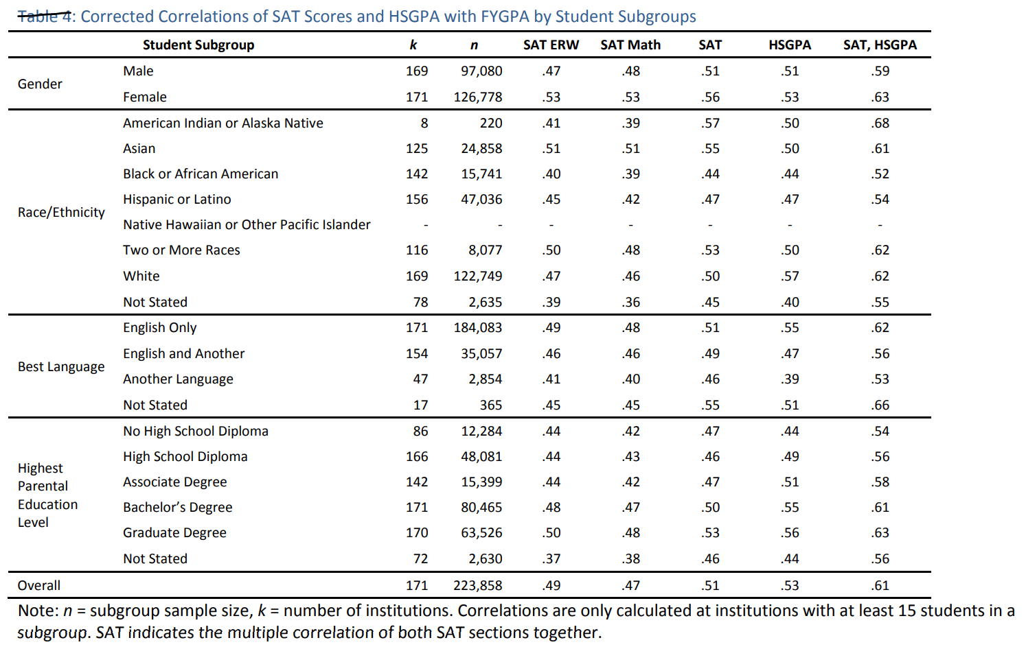
The correlations of SAT scores and HSGPA with FYGPA are both about 0.50, with some variation between demographic groups. It takes a few hours to complete the SAT, while HSGPA is based on several years' worth of assessments, yet the validities are the same. This highlights the extreme economy of cognitive ability testing, especially as the criterion variable, FYGPA, is, in a sense, the same variable as HSGPA, only remeasured. However, the combined validity of the SAT and HSGPA is about 0.60, indicating that they are not redundant with each other.
Another analysis in the validity study dealt with prediction errors. The following figure shows how much the FYGPA of various racial/ethnic groups was over- or underpredicted by SAT scores and HSGPA in relation to a prediction equation based on all groups. It can be seen that white and Asian FYGPAs are underpredicted while there is overprediction for the other groups.

Goodhart's law is an adage stating that "When a measure becomes a target, it ceases to be a good measure". With reference to that idea, it has been argued that because of the importance of the SAT in college admissions, it measures only the amount of opportunities and resources that a student has for preparing and practicing for the test, rather than his or her ability to do college-level work. What the validity data demonstrate is that whatever extraneous influences there are on the SAT, it is far from true that they deplete the test of its validity. (Nor does the 2017 redesign seem to have changed the validity of the test. A 2008 study of the previous test version reported essentially identical results.)
However, I do not think the College Board's validity study is informative about differential validity, or over- and underprediction. The differences between groups that were found do not show that the predictive power of the SAT depends on, say, race or ethnicity as such. This is because the reported results are influenced by a number of confounders, and the authors exerted very little effort to control for them. Other than measurement invariance (which is taken up in the next chapter), the most important issues are:
- There is no proper adjustment for college selectiveness. The available data would have allowed for a much more informative analysis. They have data from 171 colleges representing a wide range of selectiveness, so a school fixed-effect design would have mitigated selection bias considerably.
- There is no adjustment for what the participants are studying. For example, white and especially Asian students are more likely to major in STEM subjects than members of other groups, yet the FYGPAs of STEM and non-STEM majors are treated the same. Differences in curriculum difficulty and grading standards are ignored.
- The predictive validity data are from the very first cohort that took the redesigned test–the high school graduating class of 2017. It was a transitional cohort in which the full effects of the test redesign were not yet evident. In particular, the Asian participation rate was unusually low, with many Asian students excluded due to taking the old SAT, and the Asian-white gap was clearly smaller than in the immediately subsequent cohorts (see Figures 1.1 and 1.2 in the first chapter). Validity data from later cohorts would be more informative with respect to group differences.
- Because SAT scores are measured with some random error, the regressions of FYGPA on test scores would not be identical across groups with different SAT means (or SDs) even if none of the other confounders were present. Overprediction in low-scoring groups and underprediction in high-scoring groups is not an anomaly but rather the expected pattern. See my discussion of Kelley's paradox for an explication of this phenomenon.
- Even if none of the above issues existed, group differences in prediction systems would still often occur. The residuals of FYGPA~SAT regressions are often correlated with race/ethnicity because groups differ in other, omitted predictors of FYGPA, such as conscientiousness, leading to differences in regressions that are unrelated to the SAT per se.
Because of data-sharing agreements with colleges, the College Board has access to extremely rich individual-level student data. This would allow for very sophisticated analyses, so it is a shame that the validity study is so simple and uninformative. An example of what could be done is given in the following figure from Sackett & Kuncel (2018) which is based on old data from the 1990s.
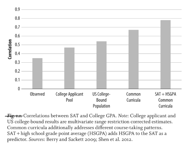
In the figure, progressively more expansive corrections for selection bias are applied to the correlation of the SAT and college GPA. The left-most correlation, 0.35, is the raw correlation without any corrections. The next one corrects for range restriction using the variability in the applicant pools of individual colleges, which increases the correlation to high 0.40s. Then, range restriction is corrected for by using the variability in the entire national SAT-taker cohort, raising the validity to over 0.50.
Especially interesting is the next correlation ("Common Curricula") which, in addition to correcting for range restriction, takes into account differences in individual course choices (the methodology is explained in Berry & Sackett, 2009), which brings the correlation closer to 0.70. Finally, HSGPA is added to the model and the final, right-most validity coefficient is almost 0.80. This analysis is useful in showing that much of the predictive validity of the SAT gets hidden away via selection processes that truncate the variance of student ability.
8. Measurement invariance
Cognitive tests are unbiased with respect to group membership (e.g., race/ethnicity) if individuals with the same true ability have the same expected test scores regardless of which group they belong to. In other words, the regressions of observed test scores on true test scores must be equal across groups. This condition of unbiasedness is called measurement invariance. If measurement invariance holds between specified groups, then the groups have had the opportunity to absorb the same knowledge and skills, and group differences reflect differences in the underlying cognitive capacity to take in information and apply it. If measurement invariance is violated, then at least some of the test score differences are due to extraneous factors that are independent of ability differences.
Note that measurement invariance is conceptually distinct from predictive invariance, which was discussed in the previous chapter. The latter concerns the relation of test scores to external variables, while the former is about the internal characteristics of tests.
In the SAT, measurement invariance is traditionally assessed by examining differential item functioning, or DIF. Educational Testing Service (ETS), which used to develop and administer the SAT on behalf of the College Board, has screened SAT items for DIF by race/ethnicity for several decades. In fact, the standard statistical procedures for detecting DIF were developed by ETS personnel to ascertain the unbiasedness of the SAT (see Dorans & Holland, 1993, for an excellent overview of the methodology).
The Appendix to the SAT Technical Manual (pp. 50–53; see also p. 44 in the Technical Manual) reports DIF analyses for several hundred items from the item pool of the current SAT. Almost every item shows only negligible DIF in all racial/ethnic groups and both sexes, and thus measurement invariance is seen to hold.
The College Board subjects all SAT item to DIF analyses before their operational use, and the results mentioned in the paragraph above are from such pretesting, i.e., the participants are not taking the test in a high-stakes setting. As far as I know, the College Board has not published any DIF results on the current SAT after 2017, and no DIF analyses based on operational administrations of the current SAT have been published at all.
I would like to see DIF results based on recent, operational, high-stakes data. DIF investigations in various smaller subgroups would be especially interesting. Some issues that could be addressed are:
- While the definition of measurement invariance does not rule out latent variance differences between groups, the variance differences in the operational SAT data between low- and high-scoring groups are sometimes so large that they raise the question whether the same traits are being measured across ability levels.
- With reference to the analysis in [Note 21], is there DIF with respect to those who take the test only because it is required in their state, and who have no intention of applying to selective colleges?
- A substantial proportion (>4%) of Asian-Americans would score above the current ceiling of the test if it was raised, and obviously the test items cannot function the same way for them as for the others, suggesting that DIF is present.
- Native American SAT scores seem to be out of step with their performance in other tests. DIF analyses would be informative.
- Is there DIF with respect to students who retake the test many times?
- How is the level of English proficiency related to DIF, especially in interaction with racial/ethnic identity?
A plausible threat to measurement invariance in the SAT are differences in preparation, motivation, and effort, or conscientiousness more generally. Cognitive ability and conscientiousness are cleanly separable constructs, with a ~0 meta-analytic correlation (Anglim et al., 2022), and should also be evaluated separately. Indeed, one of the traditional virtues of the SAT is that it has enabled colleges to tap into the "lazy but clever" quadrant of the von Manstein matrix. If changes in the test and ever-intensifying test prepping efforts have made the SAT more and more a test of conscientiousness in addition to smarts, it has lost some of this virtue.
Asian students stand out not only in terms of their test scores, but also their work ethic. For example, Asian-American high-schoolers spend an average of 2 hours and 14 minutes a day on homework, while the averages for white, Hispanic, and black students are 56 minutes, 50 minutes, and 36 minutes, respectively (Dunatchik & Park, 2022). Therefore, to the extent that practice improves SAT performance, Asians would be the most likely to put in the hours to get ahead. Byun & Park (2012) found that Asian-American students, and especially those of East Asian descent, were more likely than others to enroll in commercial SAT preparation courses, while black students were the most likely to hire private SAT tutors; whites and Hispanics were less likely than Asians and blacks to engage in these forms of SAT coaching.
That practice would improve SAT scores is not surprising as such. Cognitive training is expected to produce gains in the practiced task and closely related tasks, or near transfer, but no generalized ability gains, or far transfer (Gobet & Sala, 2023; Arendasy et al., 2016). Research on the SAT and the ACT generally suggests that coaching results in test score gains of small magnitude (Briggs, 2004; Moore et al., 2018). Could the extranormal gains of Asian students in the SAT since 2017 be due to the test becoming more amenable to coaching? That is possible but no direct evidence for it exists.
9. Discussion
After analyzing racial and ethnic differences in the SAT over the last few decades, with a special focus on what has happened in recent years, my main conclusions are the following:
- Racial/ethnic differences in the SAT are largely coterminous with IQ differences. There are some exceptions to this pattern, however, especially when it comes to Asian-Americans and Native Americans in recent years.
- The current version of the SAT that was first taken by the high school class of 2017 favors Asians compared to earlier tests. The test redesign appears to have boosted Asian total score performance by about d = 0.20 in relation to whites and others. This conclusion is supported by several lines of evidence, such as:
- In the national SAT time series, Asians had been slowly and steadily gaining on whites for decades, but after 2017 the gains accelerated considerably.
- In states where SAT participation remained at the same level before and after 2017, the Asian-white gap suddenly grew by about d = 0.20 after the new SAT was introduced.
- Before 2017, the Asian-white SAT gap was similar to the gap seen in other IQ tests. After 2017, the SAT gap has grown to be substantially larger than in other tests.
- The causes of the larger than expected Asian gains are unknown. Changes in item contents and scoring may have made the test more coachable, but no hard evidence for this exists.
- Native Americans are the worst-performing racial/ethnic group in the SAT these days. The SAT appears to underestimate the cognitive ability of Native Americans compared to other groups because they perform substantially better in other tests (e.g., SEDA and NAEP).
- In the national SAT data, blacks and Hispanics have gained modestly on whites after 2017. However, these gains are not observed in states where SAT participation has remained constant. The apparent gains are probably explainable by selection bias, viz., changes in the size and composition of the national test-taker cohorts. Black-white and Hispanic-white SAT gaps in states where SAT participation is universal are very similar to gaps in other IQ tests.
- I used publicly available summary data on the SAT in my analyses, but the most informative analyses would require individual-level data to which only the College Board has access. If the College Board published predictive validity and DIF analyses using recent operational, high-stakes data and more thoughtful methods than before, it could greatly clarify several of the above findings.
Why are racial/ethnic differences in the SAT important? For one thing, selective US colleges have long faced a problem whereby a disproportionately large share of their best-qualified applicants are Asian, while few are black or Hispanic. This makes it impossible to select applicants so that the student demographics would meet the demands of "diversity", as commonly understood, except by engaging in racial discrimination. The College Board appears to have exacerbated this problem by redesigning the SAT to especially favor Asians.
Recently, the trend in colleges has been towards "test-optional" and "test-blind" admissions. The first means that you are not required to submit test scores but they will be considered if you do, while the second means that test scores would be ignored even if you submitted them. This is, of course, in large part about trying to minimize the impact on admissions of the racial and ethnic differences in intelligence and academic ability that the SAT and the ACT so plainly reveal. Selective colleges are always devising new ways to boost the enrollment of lower-performing minority students, mainly blacks and Hispanics, in the face of legal and political challenges to race-conscious admissions. After the recent Supreme Court rulings on affirmative action, it seems that they are in a pickle.
Even with their limitations discussed in this post, standardized tests are the least biased of all the factors considered in selecting students. Test items are screened for racial/ethnic and gender bias, but there are no corresponding procedures for eliminating biases in high school transcripts, personal essays, recommendation letters, interviews, or extracurriculars. Opposition to tests is therefore fundamentally about making the admission process more biased so as to enable the preferential treatment of favored demographic groups. Aside from the issue of fairness, the elimination of testing results in efficiency losses as the best educational resources are not allocated to those with the most to gain from them. Meanwhile, the lowering of standards degrades the quality of educational institutions for all.
However, racial/ethnic preferences cannot make ability differences go away, so another reason why understanding racial and ethnic gaps in the SAT is crucial is because they are a guide to the composition of the country's cognitive elite in the 21st century. Asians are increasingly overrepresented in many prestigious occupations. It has been posited that a "bamboo ceiling" prevents Asians from reaching the most senior positions in American status hierarchies despite their strong abilities and credentials, but, at most, this seems to be true only of East Asians. As shown by Lu et al. (2020), South Asians have no trouble breaking through the bamboo ceiling, perhaps because they are more likely than East Asians to possess personality characteristics that Americans like to see in their leaders. With their numbers swelling, South Asians are poised to acquire a position as a dominant minority in both commercial and intellectual endeavors similar to the one that Jews have had in America for several generations, especially as Jewish dominance appears to be on the wane due to demographic changes. The dearth of attention paid to racial/ethnic trends in SAT scores is regrettable given their importance for understanding elite formation.[Note 26]
A new, digital version of the SAT will replace the current paper-and-pencil test in 2024. It will be interesting to see what the racial/ethnic gaps in it look like. Hopefully, the College Board will publish detailed analyses of the new test using operational data.
In this post, I have studied racial and ethnic differences in the SAT from a wide variety of perspectives, but the topic is big and there are several open questions. I have made my data and code available, and would be happy to see others extend my analysis, and explore hypotheses that I have not considered.
Notes
1. A good definition of intelligence test items is provided by Guttman & Levy (1991, p. 82):
Of course, the mere fact that the items of a test were drawn from the universe of intelligence test items, as defined above, does not necessarily mean that it is a good intelligence test. Several additional requirements must be met for the test to be adequate for measuring intelligence in a particular population. For example, the item difficulties must span a range wide enough to assess everyone's ability, and measurement invariance must hold across the groups in which the test is used (meaning that individuals with the same level of latent ability must have the same expected test scores regardless of what group they belong to).
2. The SAT was "recentered" in 1995. Dorans (2002) described this process:
For a variety of reasons dealing with score interpretation and psychometrics, the original SAT scales were replaced in April 1995 by new recentered scales [...]. The most salient reason for this change lies in the critical importance of the reference group to the universal meaning of score scales such as the SAT. The original SAT scales derived their universal meaning from a 1941 Reference Group of slightly more than 10,000 test takers. In this group, the expected SAT scores on Verbal and Math were 500. Recentering replaced this 1941 Reference Group with the 1990 Reference Group.
The 1990 Reference Group consisted of 1,052,000 students who took the SAT in 1990. Because the SAT-takers of 1990 were a much larger and less cognitively selected group than the 1941 Reference Group, their mean scores on the original scale were 424 (verbal) and 476 (math). The means of the 1990 cohort were adopted as the midpoints (i.e., 500) of the recentered verbal and math scales. Besides changing the means, the recentering fixed certain scoring issues at the high end of the scales, which Dorans (2002) described in this way:
[T]he top portions of the SAT raw-to-scale were consistently characterized by large gaps between raw scores and scaled scores. New editions of the test, especially for SAT V, were not scaling out to 800. In other words, a perfect raw score would correspond to a 760 or 770 or 780. The score reporting policy was to award an 800 to a perfect raw score. Hence the top score would be an 800, but one omission out of 85 items might cost a student 30 to 40 points.
After the recentering perfect SAT scores became easier to attain as they no longer required perfect raw scores.
All the pre-1995 data that I use in this post have been converted to the recentered scale.
3. Regardless of correlations between sections, the mean of the sum of the individual math and verbal (and writing) scores equals the sum of the means of the individual scores, assuming that the individual scores have a joint normal distribution (see here). This distributional assumption cannot be strictly true, and it is unknown whether this substantially biases the calculation of total score means. However, the College Board has reported total score means together with math and verbal means since 2017, and they seem to always be within a single point of the sum of the math and verbal means. This indicates either that the simple sum estimates the total score mean with very little bias, or that the College Board actually calculates the total score means by summing the math and verbal means (i.e., without using individual-level data).
4. The redesigned SAT was first administered in March 2016. However, in accordance with how SAT administrations are dated throughout the post, I consider it to have been introduced in 2017. This is because the high school graduating class of 2017 was the first that generally took the redesigned version.
5. Colleges accepted both the old SAT and the new SAT in 2017. Many students who had prepared for the old test and taken it, possibly multiple times, probably chose to not take the new test. This may explain the drop in the number of reported Asian test-takers in 2017–that year's College Board report includes only those who took the new test.
6. Institutional changes may explain some of the vagaries of the redesigned SAT. The College Board owns the SAT brand, but the design and administration of the test was traditionally outsourced to Educational Testing Service. After David Coleman became president of the College Board in 2012, the design of the SAT was moved in-house, and a revised test was developed and published within a few years. ETS still does contract work for the College Board, though, and the division of labor with respect to the SAT between the two is unclear.
7. Asians and Pacific Islanders were grouped together until 2016, but their splitting into separate groups explains little of the recent Asian divergence. There are about 50 Asian SAT-takers to every Pacific Islander SAT-taker, so the pooled category is almost indistinguishable from the Asian-only category. Since 2016, the aggregate Asian/Pacific Islander total score mean has been 4 to 6 points lower than the Asian-only total score mean.
R code to compute differences between Asian/Pacific Islander means and Asian means
sat1987to2022[sat1987to2022$Group=="Asian" & sat1987to2022$Year>2015,]$Total_Mean-sat1987to2022[sat1987to2022$Group=="Asian/Pacific Islander" & sat1987to2022$Year>2015,]$Total_Mean
8. Because of changes in the SAT and in what statistical information about it is made publicly available, the estimation of standardized total or composite score gaps between groups requires different methods in different time periods:
- Gaps prior to 2002 could not be estimated because of lack of data.
- Gaps in 2002–2005 were estimated with Cohen's d after using a formula for the variance of the sum of bivariate normal variates, together with a correlation between math and verbal sections based on data from a 2015 concordance study.
- Gaps in 2006–2016 were calculated by using a formula for the variance of the sum of several multivariate normal variates together with correlations between SAT sections obtained from the above-mentioned concordance study, and finally using Cohen's d.
- Gaps in 2017–2022 were calculated by first estimating SDs using methods for interval-censored distributions, and then using Cohen's d.
I will begin with the years 2006–2016 when the SAT had three sections: Critical Reading (CR), Math, and Writing (W). To calculate within-group SDs and standardized gaps for the composites of those three scores, the formula for the variance of the sum of two correlated, jointly normal variables A and B can be used:

Thus for the sum of CR and Math, the equation would be:

By induction, the variance of the sum of the three, presumably jointly normal, SAT sections is then:

The SD of the composite is obtained by taking the square root of the variance. Note that the covariance of A and B can always be written as a function of the SDs of A and B and their intercorrelation, r:

The SDs of the three sections for each group for each year are available in the College Board's reports, so the only missing pieces of information are the correlations between the sections. In 2015, a concordance study of the old SAT (i.e., the 2006–2016 version) and the revised (2017–) SAT was conducted. A sample of 8677 high-schoolers took both tests. The correlation matrix of the test sections and their composites looked as follows, with raw correlations below the diagonal and correlations after reweighting the sample to match the demographics of the typical complete SAT cohort above the diagonal (source: p. 321 here; see also pp. 114–117 in the Technical Manual):
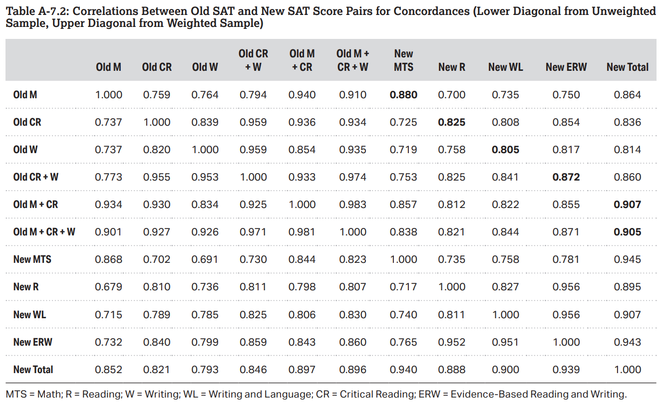
In the reweighted sample, the CR-Math, CR-W, and Math-W correlations are 0.759, 0.839, and 0.764, respectively. On the assumption that race/ethnicity or year do not moderate these correlations, they can be used to calculate SDs for the total scores in 2006–2016. The variance formula used is:

The square root of that equals the SD of the composite. Cohen's d was then used to calculate the gaps for each year.
In the absence of better data, I assumed that the pre-2006 Verbal-Math correlation equaled the Math-CR correlation in the 2015 concordance study discussed above. This is probably justifiable by the fact that the Critical Reading and Math sections of the 2006–2016 SAT are equivalent to the pre-2006 Verbal and Math sections, the Writing section having been an add-on to the old test. In any case, variation in the value of the correlation within a realistic range has little effect on d values. For the 2002–2005 period, I estimated the variances of the composite/total scores with the following formula which is based on the formula for the variance of the sum of two variables discussed at the start of this note:

The within-group verbal and math SDs/variances are available in the College Board reports for each group and each year, while the constant 0.759 is the CR-Math correlation. The square root of the composite variance equals the composite SD. Cohen's d was used to calculate the gaps.
The College Board has not reported within-group SDs for the SAT after 2016, but it does make available information on racial/ethnic SAT distributions in the form of test score bins. For example, in the 2022 national report, the total score distributions are presented in the following way:

When the full distribution of a variable is unobserved but the proportions of data points that fall into known ranges of values are known, as in here, the data are interval censored. If the assumption is made that the data follow a specific parametric distribution, it is possible to infer the full distribution from interval-censored data. When estimating how the variable would be distributed without censoring, the unobserved true values are assumed to have a certain distribution, and a likelihood function is constructed and (iteratively) maximized to find the parameters of the distribution that are the most probable given the observed data. In the case of SAT data, a reasonable starting point is that the test score distributions are normal within each race or ethnicity. The normal distribution is defined by two parameters, mean and variance, and the task is therefore to find, separately for each group and each year, means and variances (and thus also SDs) that are the most probable given the observed, censored data.
I used the fitdistrplus R package to estimate uncensored SAT score distributions from binned distributions. The procedure is simple. First, you need a data frame with variables called left and right, which represent the lower and upper bounds of each bin. For each individual, the data frame has a row indicating the bounds between which his or her test score is located. The data frame for a toy dataset of interval-censored SAT total scores for ten individuals looks like this:
left_right_df <- read.csv(text="left,right
600,790
600,790
800,990
800,990
1000,1190
1000,1190
1000,1190
1200,1390
1200,1390
1200,1390")
The mean and SD that are the most probable for those data, assuming a normal distribution, can then be obtained with the command:
fitdistcens(left_right_df, dist = "norm")
which produces the following results:
Fitting of the distribution ' norm ' on censored data by maximum likelihood
Parameters:
      estimate
mean 1034.9645
sd    212.8287
It is straightforward to extend the method to situations where the distribution is also censored from the left (floor effect) or the right (ceiling effect). In that case, you simply replace the minimum and/or maximum values of the observed distribution with NAs in the left-right data frame (e.g., for SAT total scores you would replace all instances of 400 and/or 1600 with NA). I do not adjust for left- or right-censoring in this post unless otherwise indicated.
After estimating the SDs in this manner, I used Cohen's d to calculate the SAT gaps for 2018–2022. The year 2017 had to be skipped because there is no information on the within-group variability of the SAT in that year's College Board report. The censored distribution method produces estimates of mean scores as well as SDs, but the mean scores used in this post are always empirical means from the College Board's reports, unless otherwise indicated. See [Note 23] for more information on the validity of the censored distribution method in the estimation of the moments of SAT distributions.
9. If r is the correlation between two tests, the standardized differences between two groups in the two tests, 


This means that the contributions of 
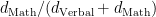
See [Note 18] for more information on the composite d formula.
10. My basic approach in this post is the aggregation of results across many samples so as to arrive at more precise estimates. The focus is on discovering robust general patterns rather than doing formal statistical tests. Nevertheless, to give some idea of the precision of the individual d values in Figure 2.1, below I report standard errors (SE) for each state and group in the high-participation states of 2009–2018.
The SE for a Cohen's d is given by the following formula (see Schmidt & Hunter, 2014, p. 421):

where the subscripted ns are the sample sizes of the two groups being compared.
The following table shows the SEs. Ns and ds being roughly constant across years, pre-2017 SEs were averaged so that the same values can be used for any of the pre-2017 cohorts.
| Asian | Black | Hispanic | Native American | |||||||||
| State | Pre-2017 | 2018 | Pre-2017 | 2018 | Pre-2017 | 2018 | Pre-2017 | 2018 | ||||
|---|---|---|---|---|---|---|---|---|---|---|---|---|
| Connecticut | 0.02 | 0.02 | 0.02 | 0.02 | 0.02 | 0.01 | 0.09 | 0.09 | ||||
The statistic for testing the significance of the difference between two d values is:
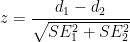
Significance is determined based on the absolute value of z. 


The p-value is about 0.000002. However, as I said, my focus is on average patterns across states rather than these individual tests.
R code for calculating SEs for high-participation states
# calculate SEs for d values in high-participation states in 2009-2018

# function for calculating standard errors for Cohen's d
cohen_d_se <- function(n1, n2, d) {
variance <- ( ( (n1 + n2) / (n1 * n2) ) + ( d^2 / (2*(n1 + n2 - 2)) ) )
return(sqrt(variance))
}

# data frame from Chapter 2 is used
high_participation_precision <- high_participation_2009to2018_gaps

high_participation_precision$SE <- with(high_participation_precision, mapply(function(n1,Total_d,year,state) cohen_d_se(n1,N[Year==year & State==state & Group=="White"],Total_d), N, d, Year, State))

se_table <- data.frame(State=unique(high_participation_precision$State), Asian_pre_2017=NA, Black_pre_2017=NA, Hispanic_pre_2017=NA, Native_American_pre_2017=NA)

# mean SEs before 2017
for(state in se_table$State) {
se_table[se_table$State==state,2:5]<-with(subset(high_participation_precision, Year<2017), sapply(c("Asian/Pacific Islander", "Black", "Hispanic/Latino", "Native American"), function(group) sqrt(weighted.mean(SE[Group==group & State==state]^2, N[Group==group & State==state]))))
}

se_table <- cbind(se_table, data.frame(Asian_2018=NA, Black_2018=NA, Hispanic_2018=NA, Native_American_2018=NA))

# SEs in 2018
for(state in se_table$State) {
se_table[se_table$State==state,6:9]<-with(subset(high_participation_precision, Year>2017), sapply(c("Asian/Pacific Islander", "Black", "Hispanic/Latino", "Native American"), function(group) sqrt(weighted.mean(SE[Group==group & State==state]^2, N[Group==group & State==state]))))
}

# reorder
se_table <- se_table[,c(1,2,6,3,7,4,8,5,9)]

# html table of SEs
library(ztable)
colnames(se_table) <- c("State", "Pre-2017", "2018", "Pre-2017", "2018","Pre-2017", "2018","Pre-2017", "2018")
cgroup <- c("", "Asian", "Black", "Hispanic", "Native American")
n.cgroup <- c(1,2,2,2,2)
se_table_html <- ztable(roundDf(
se_table,2),zebra=2,zebra.color="#d4effc;", caption="Standard errors of standardized gaps in SAT total scores in high-participation states in 2009–2016 (averaged) and 2018, White reference group", caption.placement="top",caption.position="l", caption.bold=TRUE, align="lrrrrrrrr",include.rownames=FALSE,colnames.bold=TRUE)
se_table_html <- addcgroup(se_table_html, cgroup, n.cgroup)
capture.output(se_table_html,file="se_table1.html")
11. The mean d values shown in Figure 2.2 were aggregated across states using N-weighted means where N is the sum of the sample sizes of the white and non-white groups being compared. In practice, this means that California and Texas with their large populations dominate the estimates. An alternate measure of central tendencies in the gaps is the median which is not affected by population size differences. The next table compares the mean and median ds in the eight moderate-participation states.
| Mean | Median | |||||
| Group | 2016 | 2018 | 2016 | 2018 | ||
|---|---|---|---|---|---|---|
| Asian | 0.22 | 0.40 | 0.28 | 0.43 | ||
Overall, the median d values are quite similar to the means, providing mostly equivalent estimates of the effect of the 2017 test redesign.
R code for comparing means and medians
# mean and median SAT total score gaps in 2016 and 2018

means_2016 <-subset(sat2016, State == "MEAN", select=c("Group", "Total_d"))[order(sat2016$Group),]
colnames(means_2016) <- c("Group", "Mean 2016")
means_2018 <-subset(sat2018, State == "MEAN", select=c("Group", "Total_d"))[order(sat2018$Group),]
colnames(means_2018) <- c("Group", "Mean 2018")
medians_2016 <- subset(sat2016, State == "MEDIAN", select=c("Group", "Total_d"))[order(sat2016$Group),]
colnames(medians_2016) <- c("Group", "Median 2016")
medians_2018 <- subset(sat2018, State == "MEDIAN", select=c("Group", "Total_d"))[order(sat2018$Group),]
colnames(medians_2018) <- c("Group", "Median 2018")
means_vs_medians <- na.omit(merge(means_2016,means_2018, all=TRUE))
means_vs_medians <- na.omit(merge(means_vs_medians, medians_2016, all=TRUE))
means_vs_medians <- na.omit(merge(means_vs_medians, medians_2018, all=TRUE))

# html table

colnames(means_vs_medians) <- c("Group", "2016", "2018", "2016", "2018")
cgroup <- c("", "Mean", "Median")
n.cgroup <- c(1,2,2)

means_vs_medians_html <- ztable(means_vs_medians,zebra=2,zebra.color="#d4effc;", caption="Mean and median SAT total score gaps in eight states with moderate participation", caption.placement="top",caption.position="l", caption.bold=TRUE, align="lrrrr",include.rownames=FALSE,size=3,colnames.bold=TRUE)
means_vs_medians_html <- addcgroup(means_vs_medians_html, cgroup, n.cgroup)
capture.output(means_vs_medians_html,file="means_vs_medians.html")
12. The standard errors of the d values in moderate-participation states in 2016 and 2018 were as follows:
| Asian | Black | Hispanic | Native American | |||||||||
| State | 2016 | 2018 | 2016 | 2018 | 2016 | 2018 | 2016 | 2018 | ||||
|---|---|---|---|---|---|---|---|---|---|---|---|---|
| California | 0.01 | 0.01 | 0.01 | 0.01 | 0.01 | 0.01 | 0.03 | 0.03 | ||||
See the previous footnote for more information on the calculation and uses of the SEs of d values.
R code for calculating SEs for moderate-participation states
# calculate SEs for d values in moderate-participation states in 2016-2018

# function for calculating standard errors for Cohen's d
cohen_d_se <- function(n1, n2, d) {
variance <- ( ( (n1 + n2) / (n1 * n2) ) + ( d^2 / (2*(n1 + n2 - 2)) ) )
return(sqrt(variance))
}

# data frame from Chapter 2 is used
moderate_participation_precision <- subset(sat_2016_and_2018, !State %in% c("MEAN", "MEDIAN"))

moderate_participation_precision$SE <- with(moderate_participation_precision, mapply(function(n1,d,year,state) cohen_d_se(n1,N[Year==year & State==state & Group=="White"],d), N, Total_d, Year, State))

se_table <- data.frame(State=unique(moderate_participation_precision$State), Asian_2016=NA, Black_2016=NA, Hispanic_2016=NA, Native_American_2016=NA)

# mean SEs in 2016
for(state in se_table$State) {
se_table[se_table$State==state,2:5] <- with(subset(moderate_participation_precision, Year==2016 & Group!="Pacific Islander"), sapply(c("Asian", "Black", "Hispanic/Latino", "Native American"), function(group) SE[Group==group & State==state]))
}

se_table <- cbind(se_table, data.frame(Asian_2018=NA, Black_2018=NA, Hispanic_2018=NA, Native_American_2018=NA))

# mean SEs in 2018
for(state in se_table$State) {
se_table[se_table$State==state,6:9] <- with(subset(moderate_participation_precision, Year==2018), sapply(c("Asian", "Black", "Hispanic/Latino", "Native American"), function(group) SE[Group==group & State==state]))
}

# reorder
se_table <- se_table[,c(1,2,6,3,7,4,8,5,9)]

# html table of SEs
library(ztable)
colnames(se_table) <- c("State", "2016", "2018", "2016", "2018","2016", "2018","2016", "2018")
cgroup <- c("", "Asian", "Black", "Hispanic", "Native American")
n.cgroup <- c(1,2,2,2,2)
se_table_html <- ztable(roundDf(
se_table,2),zebra=2,zebra.color="#d4effc;", caption="Standard errors of standardized gaps in SAT total scores in moderate-participation states in 2016 and 2018 (White reference group)", caption.placement="top",caption.position="l", caption.bold=TRUE, align="lrrrrrrrr",include.rownames=FALSE,colnames.bold=TRUE)
se_table_html <- addcgroup(se_table_html, cgroup, n.cgroup)
capture.output(se_table_html,file="se_table2.html")
13. The pre-2017 mean d values for the high-participation states were obtained by first calculating unweighted within-state means across years, and then using the mean Ns (across years) of each state to calculate N-weighted averages across states. The 2018 means for the high-participation states, and both the 2016 and 2018 means for the moderate-participation states are N-weighted averages across states. N in this context is the sum of the sample sizes for the focal (i.e., non-white) and reference (i.e., white) groups.
I use N-weighting to aggregate d values in Chapter 2 because there are data from only a small number of states, and many of the samples are quite small. In Chapter 3 I use random effects inverse variance weights instead because that is theoretically preferable, and there are more data from more states, enabling more reliable estimates of the between-state variances required for calculating the inverse variance weights. In Chapter 3 I am also interested in estimating what the gaps would be in random, unselected samples of high-schoolers, while in Chapter 2 the focus is on differences in the gaps before and after 2017, rather than the size of the gaps per se. The weights chosen also serve these purposes.
14. The weighting problem is the following. I have SAT results from eleven high-participation states. I want to aggregate them so as to approximate, with as little bias as possible, the results that would be obtained if we could have a random sample of high school graduates from all 50 states (+ DC) take the SAT. Random effects inverse variance weights appear to me to be a reasonable solution to this problem.
Random effects meta-analysis is based on the assumption that the sample estimates may not all be estimates of the same population value, but rather that there is an underlying normal distribution of parameter values, and that the meta-analytic mean value is an estimate of the mean of that distribution. The difference to fixed effect meta-analysis is that in the latter it is assumed that each of the sample estimates being aggregated is an estimate of the very same population value. In the fixed effect model the weights that samples receive are strongly proportional to sample sizes, whereas they are usually more evenly distributed between samples in the random effects model. The weights of the random effects model are a function of both the variances of the individual sample estimates, and the differences between the individual sample estimates. If there is no between-sample variance beyond that due to random sampling error, the random and fixed models are the same.
When aggregating SAT means across high-participation states, the random effects model makes more sense because there is no reason to believe that the states with the largest populations necessarily have the most nationally representative populations for each race/ethnicity, i.e., they do not "deserve" to contribute inordinately to the meta-analytic mean estimates that are supposed to reflect the performance of American high schoolers in general. On the other hand, it is not unreasonable to assume that the SAT means of each group are roughly normally distributed across states.
To illustrate the difference between the fixed and random effects models, let's look at the weight assigned to Florida's Hispanics in each model. In the fixed effect model, the relative weight that Florida Hispanics get in the calculation of the overall Hispanic SAT mean is about 40 percent which is close to 43 percent, the proportion of Hispanics in the high-participation state sample who are from Florida. In the random effects model, however, the relative weight given to Florida Hispanics is only about 9 percent. This downweighting of Florida Hispanics is reasonable because they are not more representative of Hispanic Americans than Hispanics from other high-participation states–in fact, they are less so because there are relatively few Mexican-Americans and many Cuban-Americans in Florida. The random-effects estimate for Hispanics is in fact close to an equal weights mean of the state estimates, a consequence of there being a great deal of between-state variation in means.
Inverse variance weighting in random effects meta-analysis is the Hedges approach which can be contrasted with the Schmidt-Hunter random-effects model where sample sizes are used as weights. The Schmidt-Hunter weights are essentially fixed-effect weights; the between-study variance is estimated in the Schmidt-Hunter scheme, too, but it is not used when calculating weights. The justification for the Schmidt-Hunter weights comes from the fact that the between-study variance is often poorly estimated, resulting in substantial bias in the inverse variance weights. I nevertheless chose the Hedges approach on the assumption that the eleven high-participation states, each with large samples for most groups, provide reasonably accurate estimates of the between-study variances.
To ascertain that my choice of weights does not lead to highly biased results, I used test scores from the Stanford Education Data Archive (SEDA) to compare different weighting schemes.
SEDA data are based on math and reading tests that states are required by federal law to administer to all students in grades 3 through 8 each year. The data consist of mean values estimated at various levels of geographic aggregation for different groups, including racial and ethnic ones. States have discretion in what the tests contain and how they are scored, so the test results are not, per se, comparable between states. However, the SEDA project uses state-level results from the NAEP assessments to place the state tests on a common scale, making them comparable across the nation.
Are SEDA results, which are based on elementary and middle school student cohorts, comparable to SAT results? The figure below shows the unweighted, pooled regression of SAT total score means on SEDA reading + math means from all grades in the eleven high SAT-participation states. Asians, blacks, Hispanics, Native Americans, and whites are included. The R2 is 81%, indicating that SEDA means predict SAT means reasonably well.

The tests that the SEDA means are based on are a bit of a hodge-podge because each state decides on its own tests. They are also not scored on a continuous scale but rather in terms of two to five performance levels, which at worst is simply a pass/fail scale. The performance categories are converted into a continuous national scale through a rather complicated process, and it seems unlikely that the SEDA tests would have a construct validity across states and groups comparable to that of tests whose design and administration is properly standardized from the get-go. The saving grace of the SEDA tests is that their sheer quantity has a quality of its own, enabling the estimation of all sorts of group differences at many levels of geographic aggregation. Moreover, the figure above suggests that despite their limitations, SEDA results are quite similar to those from higher-quality tests such as the SAT.
Another limitation of SEDA is that it does not contain SDs for racial/ethnic groups within states. The SEDA scale is standardized in relation to the mean and variability of all groups nationally, and differences between groups are expressed in terms of that variability. (This refers to what is called the CS scale. SEDA also has the GCS scale which is based on grade levels. I use only the CS scale in my analyses.) This means that it is difficult to compare the magnitude of group differences in the SEDA to other tests. However, I am using SEDA only to test different meta-analytic weighting schemes, and for this purpose, the lack of within-group SDs does not matter.
I calculated national SEDA means for each race/ethnicity as N-weighted means across all states (including DC). To the extent that the sample sizes for groups and states are proportional to the cohort sizes (i.e., data missingness is random), this should yield reasonably unbiased estimates of national means for each group. Then I compared four different aggregation methods across the eleven states so as to find out which method gives the best estimates of the national means. The mean absolute deviation and its square between a given 11-state test score aggregate and the respective national mean were used to compare the methods. The four methods are:
- N-weighting. Weighting by sample size is the Hunter-Schmidt approach to meta-analysis.
- Fixed effect inverse variance weights. The weight given to a sample is proportional to the inverse of the sample variance.
- Random effects inverse variance weights. The weight given to a sample is proportional to the inverse of the sample variance, but the sample variance is calculated as the sum of the individual sample variance and the between-samples variance, with REML used to estimate the latter.
- The median is a robust, non-parametric measure of central tendency.
The next table shows the national SEDA means across five race/ethnicity groups together with four different sets of averages calculated based on SEDA data from the eleven high SAT-participation states. All values are expressed on the SEDA scale whose national mean and SD are 0 and 1, respectively.
| Average in eleven states | |||||||
| Race/ethnicity | National mean | N-weights | Inv var FE | Inv var RE | Median | ||
|---|---|---|---|---|---|---|---|
| Asian | 0.55712 | 0.67602 | 0.58081 | 0.52925 | 0.51722 | ||
To evaluate how good the four methods are in estimating the national means, I calculated the absolute deviations and squared deviations of the different state-level estimates from the national means. The absolute deviations have the advantage of being on the same scale as the original values. The squared deviations have the advantage of giving more weight to larger deviations, penalizing large (absolute) errors more than small ones. The next two tables show these deviations and their mean values across methods.
| Race/ethnicity | N-weights | Inv var FE | Inv var RE | Median |
|---|---|---|---|---|
| Asian | 0.11890 | 0.02369 | 0.02787 | 0.03990 |
| Race/ethnicity | N-weights | Inv var FE | Inv var RE | Median |
|---|---|---|---|---|
| Asian | 0.01414 | 0.00056 | 0.00078 | 0.00159 |
The fixed-effects inverse variance weighted estimates have the smallest mean absolute deviation from the national means. The mean bias is about 5 percent of the pooled national SD, which is quite good. The median and random effects inverse variance weighted estimates are almost as good on this metric, while the N-weights are clearly inferior, with a mean bias of about 9 percent of the national SD.
Looking at the mean squared errors, the random effects inverse variance weighted estimates are the best, but the fixed effect inverse variance weights are nearly as good. The median is slightly worse than those, while the N-weights are clearly worse.
Based on these comparisons of the SEDA averages, I think the random effects inverse variance weights are a reasonable choice for the calculation of SAT means across the eleven high-participation states. While the fixed effect weights appear to be as good, if not better, in these comparisons, the difference is small. Importantly, the fixed effect assumption that the true means are the same across states is clearly incorrect in the SAT data–for example, the gap of 323 points between whites in DC and West Virginia is certainly not an artifact of sampling error. The random effects assumption that there is a distribution of different true SAT means across states is correct, and the fact that when the between-state variance is large the estimates tend towards equally-weighted means makes the random effects estimator more robust to influential outliers than the fixed effect estimator.
I also calculated mean SDs across states using inverse variance weights. First, I converted the SDs to variances, and then used the following formula to estimate their standard errors (see here for more information on the formula):
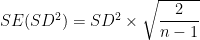
where n is the sample size. The variance of the sampling distribution is the square of the standard error. The variances for each state and their sampling variances were used as inputs to calculate inverse variance weighted random effects mean variances across states, which were then converted back to SDs.
For comparative purposes, below are the unstandardized means and SDs and standardized gaps calculated from Table 3.2 using the four methods. However, as said, the random effects inverse variance ones are my estimates of choice.
| Asian | Black | Hispanic | Native American | Pacific Islander | White | |||||||||||||
| Method | Mean | SD | Mean | SD | Mean | SD | Mean | SD | Mean | SD | Mean | SD | ||||||
|---|---|---|---|---|---|---|---|---|---|---|---|---|---|---|---|---|---|---|
| N-weights | 1163 | 226 | 884 | 162 | 950 | 183 | 860 | 158 | 900 | 175 | 1053 | 193 | ||||||
| Method | Asian | Black | Hispanic | Native American | Pacific Islander |
|---|---|---|---|---|---|
| N-weights | 0.56 | -0.90 | -0.54 | -1.00 | -0.79 |
R code for analyzing SEDA
# read SEDA data
seda <- read.csv("https://stacks.stanford.edu/file/druid:db586ns4974/seda_state_pool_cs_4.1.csv")

# national racial/ethnic means in SEDA
seda_race <- subset(seda, subcat=="race" & gap==0 & subgroup!="mtr" & stateabb != "PR")
seda_national_means <- data.frame(Group=unique(seda_race$subgroup), Mean=sapply(unique(seda_race$subgroup), function(group) weighted.mean(subset(seda_race, subgroup==group)$cs_mn_avg_ol,subset(seda_race, subgroup==group)$tot_asmts,na.rm=TRUE)))

# SEDA results from high SAT participation states
seda_sat_states <- subset(seda, subcat=="race" & gap==0 & subgroup!="mtr" & stateabb %in% c("CO", "CT", "DE", "DC", "FL", "ID", "IL", "ME", "MI", "RI", "WV"))

seda_sat_states <- seda_sat_states[order(seda_sat_states$sedafipsname, seda_sat_states$subgroup),]
seda_sat_table <- with(seda_sat_states, data.frame(State=unique(sedafipsname),
Asian_Mean = cs_mn_avg_ol[subgroup=="asn"], Asian_N = tot_asmts[subgroup=="asn"], Asian_SE = cs_mn_avg_ol_se[subgroup=="asn"],
Black_Mean = cs_mn_avg_ol[subgroup=="blk"], Black_N = tot_asmts[subgroup=="blk"], Black_SE = cs_mn_avg_ol_se[subgroup=="blk"],
Hispanic_Mean = cs_mn_avg_ol[subgroup=="hsp"], Hispanic_N = tot_asmts[subgroup=="hsp"], Hispanic_SE = cs_mn_avg_ol_se[subgroup=="hsp"],
Native_American_Mean = cs_mn_avg_ol[subgroup=="nam"], Native_American_N = tot_asmts[subgroup=="nam"], Native_American_SE = cs_mn_avg_ol_se[subgroup=="nam"],
White_Mean = cs_mn_avg_ol[subgroup=="wht"], White_N = tot_asmts[subgroup=="wht"], White_SE = cs_mn_avg_ol_se[subgroup=="wht"]
))

# data frame to analyze SAT versus SEDA in 11 states
library(reshape2)
seda_ggplot <- melt(seda_sat_table[,c(1,2,5,8,11,14)], id.vars=c("State"))
seda_ggplot$variable <- gsub("_Mean", "", seda_ggplot$variable)
seda_ggplot$variable <- gsub("_", " ", seda_ggplot$variable)
seda_ggplot$State <- gsub("Of Columbia", "of Columbia", seda_ggplot$State)
sat_ggplot <- melt(subset(high_participation_2020_master_table,Test=="Total")[,c(2,3,6,9,12,18)], id.vars=c("State"))
sat_ggplot$variable <- gsub("Hispanic_Latino","Hispanic",sat_ggplot$variable)
sat_ggplot$variable <- gsub("_"," ",sat_ggplot$variable)
colnames(seda_ggplot) <- c("State", "Group", "SEDA_Total")
colnames(sat_ggplot) <- c("State", "Group", "SAT_Total")
sat_seda_ggplot <- merge(sat_ggplot,seda_ggplot,all=TRUE)

# regression SAT~SEDA
summary(lm(data=sat_seda_ggplot, SAT_Total~SEDA_Total))

# graph of SAT~SEDA regression
library(ggplot2)
ggplot(data=sat_seda_ggplot, aes(x=SEDA_Total, y=SAT_Total,label=State,color=Group))+
geom_text(show.legend = FALSE, size=2, aes(color=Group))+
geom_smooth(se=FALSE,method="lm",aes(color=NULL))+
theme_classic()+
labs(caption="Regression of SAT total score means on SEDA total score means in 11 states", x="SEDA reading + math mean", y = "SAT total mean")+
scale_color_manual(values=c("orange", "black", "#009E73", "brown1", "purple"), name = "Race/ethnicity", guide = "legend")+
theme(plot.caption = element_text(hjust = 0, margin = margin(t = 15), size = 15))+
annotate("text", x = -0.5, y = 1050, label = bquote(R^2~"= 81%"), size = 5, color = "blue", fontface = "bold")
ggsave("sat_seda.png", height=5.4, width=9.9, dpi=300)

summary(lm(data=sat_seda_ggplot, SAT_Total~SEDA_Total))

library(metafor)
seda_sat_states_aggregates <- data.frame(Group=c("Asian", "Black", "Hispanic", "Native American", "White"),
N_weighs=sapply(seq(2,14,3), function(i) weighted.mean(seda_sat_table[,i], seda_sat_table[,i+1])),
Inverse_var_FE = sapply(seq(2,14,3), function(i) rma(yi=seda_sat_table[,i], sei=seda_sat_table[,i+2], method="FE")$beta),
Inverse_var_RE = sapply(seq(2,14,3), function(i) rma(yi=seda_sat_table[,i], sei=seda_sat_table[,i+2])$beta),
Median = sapply(seq(2,14,3), function(i) median(seda_sat_table[,i])),
National_mean = seda_national_means$Mean
)

# html table of SEDA aggregates
library(ztable)
seda_aggregates <- seda_sat_states_aggregates[,c(1,6,2:5)]
colnames(seda_aggregates) <- c("Race/ethnicity", "National mean", "N-weights", "Inv var FE", "Inv var RE", "Median")
cgroup <- c("", "", "Average in eleven states")
n.cgroup <- c(1,1,4)
seda_aggregates_table <- ztable(roundDf(seda_aggregates,5),zebra=2,zebra.color="#d4effc;", caption="SEDA averages", caption.placement="top",caption.position="l", caption.bold=TRUE, align="lrrrrr",include.rownames=FALSE,size=3,colnames.bold=TRUE)
seda_aggregates_table <- addcgroup(seda_aggregates_table, cgroup, n.cgroup)
capture.output(seda_aggregates_table,file="seda_averages.html")

# calculate MSEs
seda_sat_states_aggregates_mse <- data.frame(seda_sat_states_aggregates$Group)
seda_sat_states_aggregates_mse <- cbind(seda_sat_states_aggregates_mse, sapply(2:5, function(i) (seda_sat_states_aggregates[,i]-seda_sat_states_aggregates[,6])^2))
colnames(seda_sat_states_aggregates_mse) <-
colnames(seda_sat_states_aggregates[,1:5])
seda_sat_states_aggregates_mse <- rbind(seda_sat_states_aggregates_mse, data.frame(Group="Mean", t(colMeans(seda_sat_states_aggregates_mse[,2:5]))))

# html table comparing MSEs
colnames(seda_sat_states_aggregates_mse) <- c("Race/ethnicity", "N-weights", "Inv var FE", "Inv var RE", "Median")
mse_table <- ztable(roundDf(seda_sat_states_aggregates_mse,5),zebra=2,zebra.color="#d4effc;", caption="Squared deviations of SEDA state averages from national means", caption.placement="top",caption.position="l", caption.bold=TRUE, align="lrrrr",include.rownames=FALSE,size=3,colnames.bold=TRUE)
mse_table <- hlines(mse_table, add = c(5))
capture.output(mse_table,file="mse.html")

# calculate MADs
seda_sat_states_aggregates_mad <- data.frame(seda_sat_states_aggregates$Group)
seda_sat_states_aggregates_mad <- cbind(seda_sat_states_aggregates_mad, sapply(2:5, function(i) abs(seda_sat_states_aggregates[,i]-seda_sat_states_aggregates[,6])))
colnames(seda_sat_states_aggregates_mad) <-
colnames(seda_sat_states_aggregates[,1:5])
seda_sat_states_aggregates_mad <- rbind(seda_sat_states_aggregates_mad, data.frame(Group="Mean", t(colMeans(seda_sat_states_aggregates_mad[,2:5]))))

# html table comparing MADs
colnames(seda_sat_states_aggregates_mad) <- c("Race/ethnicity", "N-weights", "Inv var FE", "Inv var RE", "Median")
mad_table <- ztable(roundDf(seda_sat_states_aggregates_mad,5),zebra=2,zebra.color="#d4effc;", caption="Absolute deviations of SEDA state averages from national means", caption.placement="top",caption.position="l", caption.bold=TRUE, align="lrrrr",include.rownames=FALSE,size=3,colnames.bold=TRUE)
mad_table <- hlines(mad_table, add = c(5))
capture.output(mad_table,file="mad.html")

# create table of averages across 11 high SAT-participation states to compare weights

weight_comparison <- as.data.frame(matrix(nrow=4,ncol=19))
colnames(weight_comparison) <- c("Method", colnames(total_score_table[,c(2:19)]))
weight_comparison$Method <- c("N-weights", "Inv var FE", "Inv var RE", "Median")

# N-weighted means
weight_comparison[1,seq(2,19,3)] <- round(sapply(seq(2,19,3), function(i) weighted.mean(total_score_table[1:11,i],total_score_table[1:11,i+2], na.rm=TRUE)),0)

# N-weighted SDs
weight_comparison[1,seq(3,19,3)] <- round(sqrt(sapply(seq(3,19,3), function(i) weighted.mean(total_score_table[1:11,i]^2,total_score_table[1:11,i+1], na.rm=TRUE))),0)

# inverse variance FE means
means_df <- sapply(seq(2,17,3), function(i) escalc(measure="MN", mi=total_score_table[1:11,i], sdi=total_score_table[1:11,i+1], ni=total_score_table[1:11,i+2]))
weight_comparison[2,seq(2,19,3)] <- round(sapply(1:6, function(i) rma(method="FE", yi, vi, data=means_df[,i])$beta),0)

# inverse variance FE SDs
sds_df <- vector(mode="list", length=6)
sapply(seq(3,18,3), function(i) sds_df[[i/3]] <<- data.frame(mi=total_score_table[1:11,i]^2, sei=total_score_table[1:11,i]^2*sqrt(2/(total_score_table[1:11,i+1]-1)), ni=total_score_table[1:11,i+1]))
sapply(1:6, function(i) sds_df[[i]] <<- escalc(measure="MN", yi=mi, sei=sei, ni=ni, data=sds_df[[i]]))
weight_comparison[2,seq(3,19,3)] <- round(sqrt(sapply(1:6, function(i) rma(method="FE", yi, vi, data=sds_df[[i]])$beta)),0)

# inverse variance RE
weight_comparison[3,2:19] <- total_score_table[12,2:19]

# medians
weight_comparison[4,seq(2,19,3)] <- round(sapply(seq(2,19,3), function(i) median(total_score_table[1:11,i], na.rm=TRUE)),0)
weight_comparison[4,seq(3,19,3)] <- round(sqrt(sapply(seq(3,19,3), function(i) median(na.rm=TRUE,total_score_table[1:11,i]^2))),0)

# Ns
weight_comparison[,seq(4,19,3)] <- weight_comparison[3,seq(4,19,3)]

# standardized gaps

# function for calculating gaps
cohen_d <- function(group1_mean, group1_sd, group1_N, group2_mean, group2_sd, group2_N)  {
s <- sqrt( ( (group1_N-1)*group1_sd^2 + (group2_N-1)*group2_sd^2 ) / (group1_N+group2_N-2) )
return (round(((group1_mean-group2_mean)/s),2))
}

weight_comparison_std <- as.data.frame(matrix(nrow=4,ncol=6))
colnames(weight_comparison_std) <- c("Method", "Asian", "Black", "Hispanic", "Native American", "Pacific Islander")
weight_comparison_std$Method <- c("N-weights", "Inv var FE", "Inv var RE", "Median")
weight_comparison_std[,2:6] <- sapply(seq(2,15,3), function(i) cohen_d(weight_comparison[,i], weight_comparison[,i+1], weight_comparison[,i+2], weight_comparison$White, weight_comparison$White_SD, weight_comparison$White_N))

# html table of means
weight_comparison_small <- weight_comparison[,c(1,2,3,5,6,8,9,11,12,14,15,17,18)]
colnames(weight_comparison_small)  <- c("Method", "Mean", "SD", "Mean", "SD", "Mean", "SD", "Mean", "SD", "Mean", "SD", "Mean", "SD")

cgroup <- c("", "Asian", "Black", "Hispanic", "Native American", "Pacific Islander", "White")
n.cgroup <- c(1,2,2,2,2,2,2)
weight_comparison_html <- ztable(roundDf(weight_comparison_small,0),zebra=2,zebra.color="#d4effc;", caption="Comparison of weighted SAT total score averages in high-participation states in 2020", caption.placement="top",caption.position="l", caption.bold=TRUE, align="lrrrrrrrrrrrr",include.rownames=FALSE,size=3,colnames.bold=TRUE)
weight_comparison_html <- addcgroup(weight_comparison_html, cgroup, n.cgroup)
capture.output(weight_comparison_html,file="weight_comparison.html")

# html table of standardized gaps

weight_comparison_std_html <-  ztable(roundDf(weight_comparison_std,2),zebra=2,zebra.color="#d4effc;", caption="Comparison of different weights for aggregated standardized SAT total score gaps in high-participation states in 2020 (White reference group)", caption.placement="top",caption.position="l", caption.bold=TRUE, align="lrrrrr",include.rownames=FALSE,size=3,colnames.bold=TRUE)
capture.output(weight_comparison_std_html,file="weight_comparison_std.html")
15. The 95 percent confidence interval for mean 


where the subscripted SDs and ns are those of the two groups. Significance is determined based on the absolute value of z. For example,
16. Data from the high-participation states are included in the national results, so the actual differences between high-participation and other states are somewhat larger than the numbers in the main text. The eleven high-participation states account for about 18 percent of the US population, and about 26 percent of the SAT-takers in 2020. The following table compares SAT total score means in high-participation states and other states in 2020.
| Group | Mean in high-participation states | National mean without high-participation states | Difference |
|---|---|---|---|
| Asian | 1155 | 1225 | -70 |
R code for comparing states
# note: data frames from Chapters 1 and 3 are reused here

national_sat_2020 <- subset(sat1987to2022, Year==2020 & Group %in% c("Asian", "Black", "Hispanic/Latino","Native American","Pacific Islander","White"), select=c("Year","Group","Total_Mean","N"))

high_participation_2020 <- subset(high_participation_2020_master_table,Test=="Total" & State=="Overall means & Total N", select=c("Asian", "Black", "Hispanic_Latino", "Native_American","Pacific_Islander","White","Asian_N", "Black_N", "Hispanic_Latino_N", "Native_American_N","Pacific_Islander_N", "White_N"))

high_participation_vs_national <- data.frame(Group=national_sat_2020$Group, t(high_participation_2020[,1:6]), round( (national_sat_2020$Total_Mean - t(high_participation_2020[,7:12])/national_sat_2020$N * t(high_participation_2020[,1:6])) / ( (national_sat_2020$N -  t(high_participation_2020[,7:12])) / national_sat_2020$N),0), row.names=NULL)

high_participation_vs_national$Difference <- high_participation_vs_national[,2]-high_participation_vs_national[,3]

colnames(high_participation_vs_national) <- c("Group", "Mean in high-participation states", "National mean without high-participation states", "Difference")

high_participation_vs_national_table <- ztable(roundDf(high_participation_vs_national,0),zebra=2,zebra.color="#d4effc;", caption="SAT total mean scores in high-participation states and other states in 2020", caption.placement="top",caption.position="l", caption.bold=TRUE, align="lrrr",include.rownames=FALSE,size=3,colnames.bold=TRUE)
capture.output(
high_participation_vs_national_table,file="table_high_participation_vs_national.html")
17. Differences in high school dropout rates are one source of (relatively minor) bias. To estimate how much racial/ethnic differences in dropout rates affect SAT gaps in the high-participation states, I need to know what the IQ gap between high school graduates and dropouts is. To this end, I used the PIAAC survey which was conducted between 2012 and 2014. It includes literacy and numeracy tests administered to a large adult sample. I selected individuals who were between 25 and 29 years old at the time of the survey. The motivation for the cut-off of 25 is that if you have not graduated high school by age 25, you are unlikely to ever do so. The cut-off of 29 is to exclude older individuals who went to school during eras when high school graduation rates were considerably lower. All races and ethnicities were pooled together, which is suboptimal, but to get sufficient sample sizes it had to be done.
I used the PIAAC Data Explorer to obtain the data. The mean literacy and numeracy scores, standard errors of the means, and SDs for the three groups labeled "Less than high school diploma", "High school diploma/some college but no degree", and "College degree or higher (associate, bachelor, doctorate)" were as follows:
| Literacy | Numeracy | |||||||||
| Age | Education | Mean | SE | SD | Mean | SE | SD | |||
|---|---|---|---|---|---|---|---|---|---|---|
| 25–29 | Less than HS diploma | 222.53 | 6.26 | 44.22 | 204.49 | 7.31 | 47.95 | |||
Because of the complex sampling design of the PIAAC, it is difficult to calculate what proportions of people are in each of the education categories. To estimate the IQ gap associated with the HS graduate/dropout dichotomy, I must, however, know at least one of these proportions. So, I used the 2007 national dropout rate of 9.3 percent from this report as the proportion for the dropout category, 16- to 24-year-old dropouts in 2007 being mostly the same cohorts as 25–29-year-olds in 2012–2014. Additionally, I used the literacy and numeracy means pooled across all education categories (282.76 and 268.48, respectively).
Assuming normality for both scales in the total population for simplicity, the literacy and numeracy means of the high school graduates, 

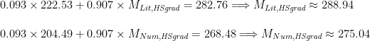
The literacy and numeracy SDs of the high school graduates, 


The standardized literacy and numeracy gaps between high school graduates and dropouts can now be calculated; they are d = 1.36 and d = 1.30, respectively. Hanushek et al. (2015) report that the correlation between the PIAAC literacy and numeracy scales is 0.85 across nations. Using the composite d formula discussed in this note, the composite literacy + numeracy gap between high school graduates and dropouts can be estimated to be d = 1.38.
Making the simplifying assumption that the gap between graduates and dropouts is the same, d = 1.38, in all groups and states, the inclusion of the dropouts would be estimated to change the average racial/ethnic gaps in the SAT total scores in the high-participation states of 2020 in the following way:
| Group | Dropout rate | Unadjusted gap | Adjusted gap |
|---|---|---|---|
| Asian | 0.02 | 0.47 | 0.50 |
All the gaps are somewhat larger in absolute size after adjustment. There are many uncertainties involved in this calculation, but the results provide some indication of the general magnitude of the dropout effects. In any case, the more conservative gaps reported in the main text are my preferred estimates.
R code for estimating the effect of HS dropouts on SAT gaps
# PIAAC data from the Data Explorer
piaac <- read.csv(text="Age,Education,Literacy_Mean,Literacy_SE,Literacy_SD,Numeracy_Mean,Numeracy_SE,Numeracy_SD
25–29,Less than HS diploma,222.53,6.26,44.22,204.49,7.31,47.95
25–29,HS diploma/some college but no degree,269.27,2.87,45.87,253.71,3.25,51.11
25–29,College degree or higher (associate/bachelor/doctorate),307.47,3.08,36.19,295.14,2.81,42.21")

# table of PIAAC results by education
library(ztable)
colnames(piaac) <- c("Age", "Education", "Mean", "SE", "SD", "Mean", "SE", "SD")
cgroup <- c("", "", "Literacy", "Numeracy")
n.cgroup <- c(1,1,3,3)
piaac_table <- ztable(roundDf(piaac, 2),zebra=2,zebra.color="#d4effc;", caption="PIAAC literacy and numeracy for different educational categories, 2012–2014", caption.placement="top",caption.position="l", caption.bold=TRUE, align="rlrrrrrr",include.rownames=FALSE,size=3,colnames.bold=TRUE)
piaac_table <- addcgroup(piaac_table, cgroup, n.cgroup)
capture.output(piaac_table,file="piaac.html")

# function for calculating gaps
cohen_d <- function(group1_mean, group1_sd, group1_N, group2_mean, group2_sd, group2_N)  {
s <- sqrt( ( (group1_N-1)*group1_sd^2 + (group2_N-1)*group2_sd^2 ) / (group1_N+group2_N-2) )
return (round(((group1_mean-group2_mean)/s),2))
}

# literacy gap between HS grads and dropouts
d1 <- cohen_d(288.94, 49.21, 907, 222.53, 44.22, 93)

# numeracy gap between HS grads and dropouts
d2 <- cohen_d(275.04, 55.06, 907, 204.49, 47.95, 93)

# composite d gap
(d1 + d2) / sqrt(2 + 2*0.85)

dropout <- data.frame(Group=c("Asian", "Black", "Hispanic", "Native American", "White"), Rate=c(0.021, 0.059, 0.078, 0.102, 0.041))

dropout$Effect <- dropout$Rate*(-1.38)
dropout$Unadjusted_gap <- as.numeric(c(total_score_gaps[12,2:5], NA))
dropout$Adjusted_gap <- with(dropout, Unadjusted_gap+Effect-Effect[5])

colnames(dropout) <- c("Group", "Dropout rate", "Effect", "Unadjusted gap", "Adjusted gap")
dropout_table <- ztable(roundDf(dropout[,c(1, 2, 4, 5)]),zebra=2,zebra.color="#d4effc;", caption="Effect of adjusting for high school dropout rates on standardized racial/ethnic SAT total score gaps in high-participation states in 2020 (White reference group)", caption.placement="top",caption.position="l", caption.bold=TRUE, align="lrrrr",include.rownames=FALSE,size=3,colnames.bold=TRUE)
capture.output(dropout_table,file="dropout.html")
18. The DAS-II gap is my own estimate based on the subtest gaps reported in this post, and the factor loadings in Table 7 of Keith et al. (2010). I used Sackett & Ellingson's (1997) equation 1 for the calculation:
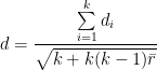
where d is a standardized difference based on a composite of multiple tests, 

The average communality of the subtests was substituted for their average intercorrelation (communality is the sum of the squares of standardized factor loadings for a given subtest, representing the proportion of variance in a subtest that is shared with other subtests).
R code for calculating the DAS-II gap
# packages that may be used
# uncomment if you don't have these installed already

#install.packages("fitdistrplus")
#install.packages("ztable")
#install.packages("reshape2")
#install.packages("ggplot2")
#install.packages("ggrepel")
#install.packages("tigerstats")
#install.packages("sjPlot")
#install.packages("scales")
#install.packages("gridExtra")
#install.packahes("grid")

# read data
das_data <- read.csv(text="Test,Asian_Mean,Asian_SD,Asian_N,Black_Mean,Black_SD,Black_N,Hispanic_Mean,Hispanic_SD,Hispanic_N,White_1_Mean,White_1_SD,White_1_N,White_2_Mean,White_2_SD,White_2_N,White_Mean,White_SD,White_N
Word Definition,53,9.55,98,46.39,9,407,47.06,8.73,432,51.3,9.6,432,51.49,9.92,432,51.39,9.76,864
Verbal Similarities,52.88,8.85,98,46.82,10.18,407,46.51,9.84,432,52.09,8.43,432,51.78,9.38,432,51.94,8.92,864
Matrices,56.68,10.58,98,46.6,10.47,407,48.3,8.97,432,51.29,9.75,432,50.93,9.8,432,51.11,9.78,864
Seq& Quant Reasoning,56.62,11.26,98,45.79,9.07,407,48.22,8.95,432,51.21,9.36,432,51.38,10.35,432,51.3,9.87,864
Pattern Construction,55.73,9.98,98,43.85,10.08,407,49.56,9.69,432,52.3,9.83,432,52.32,10.93,432,52.31,10.39,864
Recall of Designs,54.39,7.9,98,45.63,9.82,407,48.92,9.37,432,51.26,9.57,432,50.92,9.7,432,51.09,9.64,864
Recall of Obj Delayed,52.22,8.44,98,47.23,10.15,407,49.63,9.47,432,50.17,9.45,432,50.52,10.22,432,50.34,9.84,864
Recall of Obj Immediate,50.12,10.1,98,45.78,11.86,407,47.66,10.64,432,50.15,10.2,432,49.66,10.99,432,49.91,10.6,864
Digits Forward,55.32,13.04,98,49.65,10.42,407,46.7,10.16,432,50.48,11.19,432,49.98,10.96,432,50.23,11.08,864
Digits Backward,54.48,10.12,98,46.43,10.52,407,48.21,9.64,432,51.02,8.99,432,49.89,9.55,432,50.45,9.27,864
Recall of Seq Order,52.22,8.61,98,46.46,10.19,407,46.71,10.03,432,51.68,9.45,432,50.63,10.07,432,51.16,9.76,864
Speed of Info Processing,53.73,9.1,98,50.39,11.5,407,49.1,9.43,432,49.85,10.06,432,50.84,10.06,432,50.34,10.06,864
Rapid Naming,52.64,9.02,98,48.24,10.58,407,48.44,9.03,432,50.94,9.52,432,50.36,10.7,432,50.65,10.13,864")

das_loadings <- read.csv(text="Test,Unresid_loading
Pattern Construction,0.758
Speed of Info Processing,0.549
Recall Sequential Order,0.784
Digits Backward,0.767
Digits Forward,0.675
Recall Objects Immediate,0.918
Recall Objects Delayed,0.784
Recall of Designs,0.718
Sequent & Quant. Reasoning,0.8
Matrices,0.727
Verbal Similarities,0.804
Word Definitions,0.781
Rapid Naming,0.66")

# function for calculating gaps
cohen_d <- function(group1_mean, group1_sd, group1_N, group2_mean, group2_sd, group2_N)  {
s <- sqrt( ( (group1_N-1)*group1_sd^2 + (group2_N-1)*group2_sd^2 ) / (group1_N+group2_N-2) )
return (round(((group1_mean-group2_mean)/s),2))
}

# calculate subtest gaps
white_asian_gaps <- sapply(1:13, function(i) cohen_d(das_data[i,"White_Mean"], das_data[i, "White_SD"], das_data[i, "White_N"], das_data[i,"Asian_Mean"], das_data[i, "Asian_SD"], das_data[i, "Asian_N"]))

# calculate overall gap
sum(white_asian_gaps) / sqrt(13 + 13*(13-1)*mean(das_loadings$Unresid_loading^2))
19. Looking at the tables in this footnote, it is apparent that Native Americans have substantially higher SEDA scores in the eleven states than nationally regardless of the weighting scheme chosen. This suggests that their SAT mean across the eleven states, low as it is, is nevertheless higher than their nationally representative SAT mean would be.
What is more, when looking at the SAT-SEDA regression graph in this footnote, it is clear that Native Americans score lower in the SAT than their SEDA scores would predict (given the prediction equation based on the pooled sample of all racial/ethnic groups). One hypothesis to explain this discrepancy is that the relative test performance of Native Americans declines after childhood. Alternatively, the decline may be cohort-specific, with younger cohorts performing less well.
SEDA data enable the testing of these age and cohort hypotheses. The table below shows SEDA reading gaps in Native Americans, calculated as Native American mean–White mean, in grades 3 through 8 for the cohort born in 2002 (which generally graduated high school in 2020, i.e., it is the cohort whose SAT scores are analyzed in Chapter 3). The other groups are included for comparison. The data are from all states, and are expressed on the SEDA scale where the pooled national mean is 0 and the pooled national SD is 1. The gaps are not directly comparable to standardized gaps in other tests because within-group SDs are not used, but the rank order of the groups is readily interpretable.
| Grade | Asian | Black | Hispanic | Native American |
|---|---|---|---|---|
| 3 | 0.11 | -0.68 | -0.59 | -0.44 |
There is no indication of declining Native American performance at older ages. Notably, Native Americans outperform blacks and Hispanics in SEDA, but not in the SAT. This suggests that the decline effect is highly age- or test-specific, appearing only in high school and perhaps only in the SAT.
The next table shows reading gaps in 8th grade across ten different cohorts born in 1995–2004.
| Birth year | Asian | Black | Hispanic | Native American |
|---|---|---|---|---|
| 1995 | 0.20 | -0.67 | -0.61 | -0.39 |
There are essentially no cohort effects in Native Americans. The other groups show more evidence of increasing (Asian, black) or decreasing (Hispanic) trends in (absolute) gaps in relation to whites. In 8th grade, Native Americans also handily outscore blacks and Hispanics in all cohorts. This deepens the mystery of why Native Americans are doing so poorly in the SAT.
R code for analyzing age and cohort effects in SEDA
# read unpooled SEDA data
seda_unpooled <- read.csv("https://stacks.stanford.edu/file/druid:db586ns4974/seda_state_long_cs_4.1.csv")

# SEDA cohort of school children born in 2002
seda_age_cohort <- subset(seda_unpooled,
subject == "rla" & (
(year == 2011 & grade == 3) |
(year == 2012 & grade == 4) |
(year == 2013 & grade == 5) |
(year == 2014 & grade == 6) |
(year == 2015 & grade == 7) |
(year == 2016 & grade == 8) ) &
stateabb != "PR")

# SEDA gaps vs. whites in the 2002 birth cohort
seda_age_effects <- with(seda_age_cohort, data.frame(Grade = 3:8,
Asian = -1*sapply(3:8, function(i) weighted.mean(cs_mn_wag[grade==i],totgyb_wag[grade==i],na.rm=TRUE)),
Black = -1*sapply(3:8, function(i) weighted.mean(cs_mn_wbg[grade==i],totgyb_wbg[grade==i],na.rm=TRUE)),
Hispanic = -1*sapply(3:8, function(i) weighted.mean(cs_mn_whg[grade==i],totgyb_whg[grade==i],na.rm=TRUE)),
Native_American = -1*sapply(3:8, function(i) weighted.mean(cs_mn_wng[grade==i],totgyb_wng[grade==i],na.rm=TRUE))
))

# grade 8 data from different SEDA cohorts
seda_grade_8 <- subset(seda_unpooled, subject == "rla" & grade == 8 & stateabb != "PR")

# SEDA gaps vs. whites in 8th grade across cohorts
seda_cohort_effects <- with(seda_grade_8, data.frame(Birth_year = unique(year)-14,
Asian = -1*sapply(unique(year), function(i) weighted.mean(cs_mn_wag[year==i],totgyb_wag[year==i],na.rm=TRUE)),
Black = -1*sapply(unique(year), function(i) weighted.mean(cs_mn_wbg[year==i],totgyb_wbg[year==i],na.rm=TRUE)),
Hispanic = -1*sapply(unique(year), function(i) weighted.mean(cs_mn_whg[year==i],totgyb_whg[year==i],na.rm=TRUE)),
Native_American = -1*sapply(unique(year), function(i) weighted.mean(cs_mn_wng[year==i],totgyb_wng[year==i],na.rm=TRUE))
))

# html table of age effects
colnames(seda_age_effects) <- gsub("_", " ", colnames(seda_age_effects))
seda_age_effects_html <- ztable(roundDf(
seda_age_effects,2),zebra=2,zebra.color="#d4effc;", caption="SEDA reading gaps across grades for the cohort born in 2002 (White reference group)", caption.placement="top",caption.position="l", caption.bold=TRUE, align="rrrrr",include.rownames=FALSE,colnames.bold=TRUE)
capture.output(seda_age_effects_html,file="seda_age_effects.html")

# html table of cohort effects
seda_cohort_effects$Birth_year <- as.character(seda_cohort_effects$Birth_year)
colnames(seda_cohort_effects) <- gsub("_", " ", colnames(seda_cohort_effects))
seda_cohort_effects_html <- ztable(seda_cohort_effects,zebra=2,zebra.color="#d4effc;", caption="SEDA reading gaps in 8th grade across cohorts (White reference group)", caption.placement="top",caption.position="l", caption.bold=TRUE, align="rrrrr",include.rownames=FALSE,colnames.bold=TRUE)
capture.output(seda_cohort_effects_html,file="seda_cohort_effects.html")
20. The correlations between ERW and Math across groups are of some interest, and can be estimated from the available summary data.
The variance of the total scores is:

The correlation is therefore:

The table below shows the correlations for each group in the high-participation states.
| State | Asian | Black | Hispanic/Latino | Native American | Pacific Islander | White |
|---|---|---|---|---|---|---|
| Colorado | 0.75 | 0.83 | 0.83 | 0.65 | 0.88 | 0.83 |
Elsewhere, the correlation has been estimated from individual-level data to be 0.781 (p. 321 here). Taking into account the imprecision caused by multiple layers of rounding and small numbers for some groups, the population correlations underlying the estimates in the table above are probably close to that magnitude across all groups. That the correlations are of the expected size also serves to validate the censored data method that I used to estimate the SDs of the SAT distributions–if the SDs are correct, the correlations computed using them should have sensible values.
R code for estimating correlations between ETW and Math
# calculate correlations between ERW and math in high-participation states in 2020

erw_math_corr <- with(subset(high_participation_2020_master_table,State!="Overall means & Total N"),
data.frame(State=State[1:11],
Asian = ( Asian_SD[Test=="Total"]^2 - Asian_SD[Test=="ERW"]^2 - Asian_SD[Test=="Math"]^2 ) /
(2 * Asian_SD[Test=="ERW"] * Asian_SD[Test=="Math"] ),
Black = ( Black_SD[Test=="Total"]^2 - Black_SD[Test=="ERW"]^2 - Black_SD[Test=="Math"]^2 ) /
(2 * Black_SD[Test=="ERW"] * Black_SD[Test=="Math"] ),
Hispanic_Latino = ( Hispanic_Latino_SD[Test=="Total"]^2 - Hispanic_Latino_SD[Test=="ERW"]^2 - Hispanic_Latino_SD[Test=="Math"]^2 ) /
(2 * Hispanic_Latino_SD[Test=="ERW"] * Hispanic_Latino_SD[Test=="Math"] ),
Native_American = ( Native_American_SD[Test=="Total"]^2 - Native_American_SD[Test=="ERW"]^2 - Native_American_SD[Test=="Math"]^2 ) /
(2 * Native_American_SD[Test=="ERW"] * Native_American_SD[Test=="Math"] ),
Pacific_Islander = ( Pacific_Islander_SD[Test=="Total"]^2 - Pacific_Islander_SD[Test=="ERW"]^2 - Pacific_Islander_SD[Test=="Math"]^2 ) /
(2 * Pacific_Islander_SD[Test=="ERW"] * Pacific_Islander_SD[Test=="Math"] ),
White = ( White_SD[Test=="Total"]^2 - White_SD[Test=="ERW"]^2 - White_SD[Test=="Math"]^2 ) /
(2 * White_SD[Test=="ERW"] * White_SD[Test=="Math"] )
))

# N-weighted mean correlations
erw_math_corr <-rbind(erw_math_corr, with(high_participation_2020_master_table, list("N-weighted mean",
weighted.mean(erw_math_corr[,2], Asian_N[1:11]),
weighted.mean(erw_math_corr[,3], Black_N[1:11]),
weighted.mean(erw_math_corr[,3], Hispanic_Latino_N[1:11]),
weighted.mean(erw_math_corr[,3], Native_American_N[1:11]),
weighted.mean(erw_math_corr[c(1:3,5:11),5], Pacific_Islander_N[c(1:3,5:11)]),
weighted.mean(erw_math_corr[,3], White_N[1:11]))))

erw_math_corr[,2:7]<-round(erw_math_corr[,2:7],2)

# html table of ERW-math correlations
colnames(erw_math_corr) <- gsub("_", " ", colnames(erw_math_corr))
colnames(erw_math_corr) <- gsub("Hispanic Latino", "Hispanic/Latino", colnames(erw_math_corr))
erw_math_corr_table <- ztable(erw_math_corr,zebra=2,zebra.color="#d4effc;", caption="Correlations between ERW and Math in high-participation states in 2020", caption.placement="top",caption.position="l", caption.bold=TRUE, align="lrrrrrr",include.rownames=FALSE,size=3,colnames.bold=TRUE)
erw_math_corr_table <- hlines(erw_math_corr_table, add = c(11))
capture.output(erw_math_corr_table,file="correlation_table.html")
21. A peculiar thing about the SAT score distributions in high-participation states in 2020 that were estimated in Chapter 3 is that as the mean scores increase, so do the SDs. The following graph shows the N-weighted regressions of SDs on mean scores based on total score data from Table 3.2, with each dot representing a racial/ethnic group in one of the eleven high-participation states:

The solid colored lines are the regression lines for each group, while the dashed black line is the regression for all groups pooled together. It can be seen that the higher the mean score of a group, the larger its SD tends to be as well. This is true both in the pooled data, and for each race/ethnicity separately. The slope of the dashed black line is 0.17, indicating that as the SAT mean score of a group increases by one point, its SD is expected to increase by 0.17 points. Thus if one group outscores another by 100 points, its expected SD is 0.17 * 100 = 17 points higher than that of the other group. The R2 value of the pooled regression is 77%, which means that SDs can be predicted from means with a rather high accuracy.
The graph shows some evidence of heterogeneity in slopes between groups, but the largest deviations from the pooled slope are seen in the smallest-N groups, and in general the statistical power to distinguish slope differences in these data is low. I will therefore assume that the slope is the same across groups, but I will investigate whether there are group differences in intercepts. Intercept differences indicate that after controlling for mean score differences, there are still systematic differences in predicted SDs between groups. In particular, given the high variance of Asians in the SAT, it is interesting to see whether their higher mean performance is sufficient to statistically explain their greater variance.
The table below shows two regression models. The first is the simple regression of SDs on means in the pooled data for the eleven high-participation states. In the second model, racial/ethnic groups are added to the regression as dummy variables, with whites as the reference group. Both models are weighted by sample size.
| Model 1 | Model 2 | |||||
|---|---|---|---|---|---|---|
| Predictors | Est | SE | adj. p | Est | SE | adj. p |
| (Intercept) | 11.71 | 12.00 | 0.333 | 26.82 | 27.98 | 1.000 |
| Mean score | 0.17 | 0.01 | <0.001 | 0.16 | 0.03 | <0.001 |
| Asian (vs. white) | 15.71 | 4.89 | 0.013 | |||
| Black (vs. white) | -4.19 | 5.07 | 1.000 | |||
| Hispanic/Latino (vs. white) | 6.32 | 3.32 | 0.310 | |||
| Native American (vs. white) | -5.96 | 9.28 | 1.000 | |||
| Pacific Islander (vs. white) | 4.86 | 20.58 | 1.000 | |||
| Observations | 65 | 65 | ||||
| R2 / R2 adjusted | 0.772 / 0.769 | 0.852 / 0.836 | ||||
Model 1 is the one illustrated by the dashed line in the figure above. In Model 2, the effect of the mean score is very similar to Model 1, while the point estimates of all the group dummies are positive, indicating that these groups tend to have higher SDs than the white reference group after controlling for the association between means and SDs. However, the dummy estimates are, except for the Asian one, rather small, and after I used the Holm method to adjust the p-values of Model 2 for multiple comparisons, only the Asian dummy was significant at the 5 percent level, as can be seen from the table.
In the eleven high SAT participation states, Asian total score means were higher than white means by 92 points, on average (see Table 3.2). Therefore, using the slope coefficient from Model 2, Asians would be expected to have an average SD 92 × 0.16 ≈ 15 points higher than whites because of whatever causes means and SDs to be associated in these data. Moreover, because the coefficient of the Asian dummy is about 16, on the whole the Asian SD is expected to be 15 + 16 = 31 points higher than the white SD. In Table 3.2, the average Asian SD is 37 points higher than that of whites, so the model predicts this SD gap reasonably well. The SD inflation of 15 points due to the higher mean performance represents a general mechanism affecting all racial/ethnic groups, while the extra variability on top of that is specific to Asians, requiring some other explanation.
The mean-variance dependence in the 2020 SAT data suggests that there is some extraneous factor correlated with mean scores that increases both means and variances. While a positive correlation between means and SDs is sometimes observed in cognitive test data, I do not think there is any necessary connection between the two. To test the generality of the phenomenon, I regressed SDs on means in the eight states with moderate participation in the SAT discussed in Chapter 2 (cf., Table 2.2). The next tables show these regressions in the 2016 and 2018 data.
| Model 3 | Model 4 | |||||
|---|---|---|---|---|---|---|
| Predictors | Est | SE | adj. p | Est | SE | adj. p |
| (Intercept) | 135.26 | 33.61 | <0.001 | 194.56 | 58.85 | 0.013 |
| Mean score | 0.10 | 0.02 | <0.001 | 0.05 | 0.04 | 0.884 |
| Asian (vs. white) | 68.80 | 5.28 | <0.001 | |||
| Black (vs. white) | 3.48 | 11.80 | 1.000 | |||
| Hispanic/Latino (vs. white) | 7.03 | 9.67 | 1.000 | |||
| Native American (vs. white) | 21.12 | 20.38 | 1.000 | |||
| Pacific Islander (vs. white) | 21.22 | 40.33 | 1.000 | |||
| Observations | 44 | 44 | ||||
| R2 / R2 adjusted | 0.309 / 0.293 | 0.902 / 0.886 | ||||
| Model 5 | Model 6 | |||||
|---|---|---|---|---|---|---|
| Predictors | Est | SE | adj. p | Est | SE | adj. p |
| (Intercept) | 97.09 | 16.86 | <0.001 | 136.10 | 51.27 | 0.067 |
| Mean score | 0.07 | 0.02 | <0.001 | 0.03 | 0.05 | 1.000 |
| Asian (vs. white) | 28.55 | 4.60 | <0.001 | |||
| Black (vs. white) | -2.57 | 8.56 | 1.000 | |||
| Hispanic/Latino (vs. white) | 4.96 | 6.85 | 1.000 | |||
| Native American (vs. white) | 8.96 | 15.07 | 1.000 | |||
| Pacific Islander (vs. white) | 2.07 | 17.44 | 1.000 | |||
| Observations | 48 | 48 | ||||
| R2 / R2 adjusted | 0.309 / 0.294 | 0.778 / 0.746 | ||||
In both 2016 and 2018, the effect of the mean scores on the SDs is non-significant once the group dummies are added to the model. This suggests that the mean-SD dependence may be limited to the high-participation states. The Asian dummies are highly significant in both years, reflecting the long-standing phenomenon of higher variability of Asians in the SAT.
I also regressed SDs on means in the national SAT cohorts from 2002 through 2022. The next table shows these regressions.
| Model 7 | Model 8 | |||||
|---|---|---|---|---|---|---|
| Predictors | Est | SE | adj. p | Est | SE | adj. p |
| (Intercept) | 93.26 | 14.81 | <0.001 | 223.91 | 24.25 | <0.001 |
| Mean score | 0.09 | 0.01 | <0.001 | -0.03 | 0.02 | 0.266 |
| Three sections | 58.49 | 7.10 | <0.001 | 114.80 | 9.90 | <0.001 |
| Asian/Pacific Islander (vs. white) | 50.05 | 2.79 | <0.001 | |||
| Black (vs. white) | -22.03 | 5.84 | 0.001 | |||
| Hispanic/Latino (vs. white) | -10.70 | 4.31 | 0.044 | |||
| Native American (vs. white) | -2.69 | 9.45 | 0.776 | |||
| Observations | 100 | 100 | ||||
| R2 / R2 adjusted | 0.918 / 0.916 | 0.983 / 0.982 | ||||
The "Three sections" variable is a dummy for the years 2006–2016 when the SAT had three sections, and its purpose is to soak up the variance associated with the third section (Writing) so as to make all years comparable. It can be seen that with group dummies in the model, mean scores do not have a significant main effect in the national data, either. As in the state-level data, the Asian dummy has a significant positive coefficient–Asians have long been more variable than others in the SAT. There is also some evidence of lower SDs in Hispanics and especially blacks when compared to whites.
The mean-SD dependence is seen in the high-participation state data, but not elsewhere. The high-participation state data differ from other data in that they include all high school graduates, including those not particularly motivated to take the test. In contrast, the data from moderate-participation states as well as the national data are essentially convenience samples strongly impacted by self-selection into participation. This readily suggests a mechanism whereby, in the high-participation states, the test-takers are split into a highly motivated contingent that has prepared carefully and aims for maximal performance in the test, and another contingent that has done little to no preparation and does not care about their test scores. This would have the effect of increasing test score variation due to construct-irrelevant reasons, meaning that differences in motivation, test-savviness, and effort would explain substantial variation in the scores unlike in samples where differences in such factors are less important. The correlation between means and SDs would exist because higher-ability subgroups are more motivated to succeed, and/or because their scores improve more from preparation and practice.
R code for analyzing the relation between SAT means and SDs
# data frames from chapters 1-3 are reused here

#install.packages("fitdistrplus")
#install.packages("ztable")
#install.packages("reshape2")
#install.packages("ggplot2")
#install.packages("ggrepel")
#install.packages("tigerstats")
#install.packages("sjPlot")
#install.packages("scales")
#install.packages("gridExtra")
#install.packahes("grid")

# rearrange total SAT means into long format for the 2020 high-participation state data

library(reshape2)

total_means <- total_score_table[1:11,c(1,2,5,8,11,14,17)]
total_sds <- total_score_table[1:11,c(1,3,6,9,12,15,18)]
total_ns <- total_score_table[1:11,c(1,4,7,10,13,16,19)]

total_means <- melt(total_means, id.vars="State")
colnames(total_means) <- c("State", "Group", "Mean")

total_sds <- melt(total_sds, id.vars="State")
colnames(total_sds) <- c("State", "Group", "SD")
total_sds$Group <- gsub("_SD", "", total_sds$Group)

total_ns <- melt(total_ns, id.vars="State")
colnames(total_ns) <- c("State", "Group", "N")
total_ns$Group <- gsub("_N", "", total_ns$Group)
total_long <- merge(total_means, total_sds, by=c("State", "Group"))
total_long <- merge(total_long, total_ns, by=c("State", "Group"))
total_long$Group <- gsub("_", " ", total_long$Group)

# plot of regression of SDs on means for 2020 high-participation state data
library(ggplot2)
ggplot(data=total_long, aes(x=Mean, y=SD, color=Group))+
geom_point(aes(size=N))+
geom_smooth(aes(weight=N), method="lm",fill = "transparent")+
geom_smooth(aes(x=Mean, y=SD, weight=N, color="All groups"), linetype="dashed", method="lm", fill = "transparent")+
scale_size_continuous(name = "Sample size", breaks=c(50,500,5000,25000,50000))+
scale_x_continuous(breaks=seq(800,1250,50))+
scale_y_continuous(breaks=seq(75,250,25))+
theme_classic()+
scale_color_manual(
    values = c("Black"="#999999", "Native American"="brown1", "Asian"="purple", "Hispanic/Latino"="#009E73", "Pacific Islander"="#F0E442", "White"="#56B4E9", "All groups"="black"))+
guides(color=guide_legend(order=1,override.aes=list(shape=c(NA,16,16,16,16,16,16),linetype=c(6,1,1,1,1,1,1))))+
labs(color="Race/ethnicity", caption="Regression of SAT total score standard deviations on mean scores by\nrace/ethnicity, high-participation states, 2020", x = "Mean score", y = "Standard deviation")+
theme(panel.grid.major = element_line(color = "gray87", linetype = "dotted"), plot.caption = element_text(hjust = 0, size=16, margin=margin(t=12)), legend.title=element_text(size=16), legend.text = element_text(size=14), axis.text=element_text(size=14), axis.title.x=element_text(size=14, margin = margin(t = 7)),axis.title.y=element_text(size=14, margin = margin(r = 7)))
ggsave("sd_on_means_high_participation_2020.png", height=5.4, width=9.9, dpi=300)

# create dummy variables
total_long$Asian <- ifelse(total_long$Group=="Asian", 1, 0)
total_long$Black <- ifelse(total_long$Group=="Black", 1, 0)
total_long$Hispanic_Latino <- ifelse(total_long$Group=="Hispanic/Latino", 1, 0)
total_long$Native_American <- ifelse(total_long$Group=="Native American", 1, 0)
total_long$Pacific_Islander <- ifelse(total_long$Group=="Pacific Islander", 1, 0)
total_long$White <- ifelse(total_long$Group=="White", 1, 0)

# run regressions
m1 <- lm(SD~Mean, weights=N, data=total_long)
m2 <- lm(SD~Mean+Asian+Black+Hispanic_Latino+Native_American+Pacific_Islander, weights=N, data=total_long)

library(sjPlot)
tab_model(m1,m2,file="sd_on_means_high_participation_2020.html", show.se=TRUE,show.ci=FALSE,dv.labels = c("Model 1", "Model 2"), string.est="Est", string.se="SE", string.p="adj. p", title="Regression of SAT total score standard deviations on mean scores and group dummies in high-participation states in 2020 (weighted by sample size)", pred.labels=c("(Intercept)", "Mean score", "Asian (vs. white)","Black (vs. white)","Hispanic/Latino (vs. white)","Native American (vs. white)","Pacific Islander (vs. white)"), p.adjust = "holm")

# regress SAT SDs on means in moderate-participation states in 2016

# create dummy variables
sat2016$Asian <- ifelse(sat2016$Group=="Asian", 1, 0)
sat2016$Black <- ifelse(sat2016$Group=="Black", 1, 0)
sat2016$Hispanic_Latino <- ifelse(sat2016$Group=="Hispanic/Latino", 1, 0)
sat2016$Native_American <- ifelse(sat2016$Group=="Native American", 1, 0)
sat2016$Pacific_Islander <- ifelse(sat2016$Group=="Pacific Islander", 1, 0)
sat2016$White <- ifelse(sat2016$Group=="White", 1, 0)

m3 <- lm(Total_SD~Total_Mean, weights=N, data=subset(sat2016, Group %in% c("Asian", "Black", "Hispanic/Latino", "Native American", "Pacific Islander", "White") & !State %in% c("MEAN", "MEDIAN")))
m4 <- lm(Total_SD~Total_Mean+Asian+Black+Hispanic_Latino+Native_American+Pacific_Islander, weights=N, data=subset(sat2016, Group %in% c("Asian", "Black", "Hispanic/Latino", "Native American", "Pacific Islander", "White") & !State %in% c("MEAN", "MEDIAN")))

tab_model(m3,m4,file="sd_on_means_moderate_participation_2016.html", show.se=TRUE,show.ci=FALSE,dv.labels = c("Model 3", "Model 4"), string.est="Est", string.se="SE", string.p="adj. p", title="Regression of SAT total score standard deviations on mean scores and group dummies in moderate-participation states in 2016 (weighted by sample size)", pred.labels=c("(Intercept)", "Mean score", "Asian (vs. white)","Black (vs. white)","Hispanic/Latino (vs. white)","Native American (vs. white)","Pacific Islander (vs. white)"), p.adjust = "holm")

# regress SAT SDs on means in moderate-participation states in 2018

# create dummy variables
sat2018$Asian <- ifelse(sat2018$Group=="Asian", 1, 0)
sat2018$Black <- ifelse(sat2018$Group=="Black", 1, 0)
sat2018$Hispanic_Latino <- ifelse(sat2018$Group=="Hispanic/Latino", 1, 0)
sat2018$Native_American <- ifelse(sat2018$Group=="Native American", 1, 0)
sat2018$Pacific_Islander <- ifelse(sat2018$Group=="Pacific Islander", 1, 0)
sat2018$White <- ifelse(sat2018$Group=="White", 1, 0)

m5 <- lm(Total_SD~Total_Mean, weights=N, data=subset(sat2018, Group %in% c("Asian", "Black", "Hispanic/Latino", "Native American", "Pacific Islander", "White") & !State %in% c("MEAN", "MEDIAN")))
m6 <- lm(Total_SD~Total_Mean+Asian+Black+Hispanic_Latino+Native_American+Pacific_Islander, weights=N, data=subset(sat2018, Group %in% c("Asian", "Black", "Hispanic/Latino", "Native American", "Pacific Islander", "White") & !State %in% c("MEAN", "MEDIAN")))

tab_model(m5,m6,file="sd_on_means_moderate_participation_2018.html", show.se=TRUE,show.ci=FALSE,dv.labels = c("Model 5", "Model 6"), string.est="Est", string.se="SE", string.p="adj. p", title="Regression of SAT total score standard deviations on mean scores and group dummies in moderate-participation states in 2018 (weighted by sample size)", pred.labels=c("(Intercept)", "Mean score", "Asian (vs. white)","Black (vs. white)","Hispanic/Latino (vs. white)","Native American (vs. white)","Pacific Islander (vs. white)"), p.adjust = "holm")

# regress total scores SDs on means in national SAT data

# create dummy variables
sat1987to2022$Asian_Pacific_Islander <- ifelse(sat1987to2022$Group=="Asian/Pacific Islander", 1, 0)
sat1987to2022$Black <- ifelse(sat1987to2022$Group=="Black", 1, 0)
sat1987to2022$Hispanic_Latino <- ifelse(sat1987to2022$Group=="Hispanic/Latino", 1, 0)
sat1987to2022$Native_American <- ifelse(sat1987to2022$Group=="Native American", 1, 0)
sat1987to2022$White <- ifelse(sat1987to2022$Group=="White", 1, 0)

# indicator for three-section SAT
sat1987to2022$Three_sections <- ifelse(sat1987to2022$Year %in% c(2006:2016), 1, 0)

m7<-lm(Total_SD~Total_Mean+Three_sections, weights=N, data=subset(sat1987to2022, Group %in% c("Asian/Pacific Islander", "Black", "Hispanic/Latino", "Native American", "White")))
m8<-lm(Total_SD~Total_Mean+Asian_Pacific_Islander+Black+Hispanic_Latino+Native_American+Three_sections, weights=N, data=subset(sat1987to2022, Group %in% c("Asian/Pacific Islander", "Black", "Hispanic/Latino", "Native American", "White")))

tab_model(m7,m8,file="sd_on_means_national_cohorts.html", show.se=TRUE,show.ci=FALSE,dv.labels = c("Model 7", "Model 8"), string.est="Est", string.se="SE", string.p="adj. p", title="Regression of SAT total score standard deviations on mean scores and group dummies in national SAT cohorts, 2002–2022 (weighted by sample size)", pred.labels=c("(Intercept)", "Mean score", "Three sections", "Asian/Pacific Islander (vs. white)", "Black (vs. white)", "Hispanic/Latino (vs. white)", "Native American (vs. white)"), p.adjust = "holm")
22. The Asian-white SAT total score gap was only 49 points in California in 2020, a small difference compared to the national data and most of the high-participation states. However, the SAT participation rate was only 67 percent in California in 2020, and a comparison of the sample sizes in the SAT to the demographics of California high school graduates indicates that, in proportional terms, Asians are about twice as likely as whites to take the SAT in California. For this reason, the results of the California Achievement Tests cannot be meaningfully compared to those of the California SAT.
Asian–white differences in the California Achievement Tests can be further analyzed by comparing standardized gaps between pairs of groups. In the table below, positive gaps indicate that an Asian group outscores whites, while negative gaps show a white advantage.
| Comparison | Reading | Math |
|---|---|---|
| Asian Indian–White | -0.02 | 0.24 |
Overall, whites have an advantage of 0.06 SDs in reading, while Asian have an advantage of 0.27 SDs in math. The reading + math composite score gap would be about 0.20, favoring Asians. For comparison, the Asian leads in the 2020 SAT in high-participation states were 0.22 in reading and writing, 0.65 in math, and 0.47 overall (see Tables 3.3, 3.6, and 3.8 in Chapter 3). Asian performance in the SAT is clearly superior to that in the California tests. In fact, in the SAT, the average Asian outperformed the white average to a greater degree than the highest-performing Asian subgroups did in the California tests. Asian performance both in terms of means and in terms of variances is much less remarkable in the California Achievement Tests than in the SAT. The testing age and the tested cohorts are not the same, but the difference is nevertheless striking, underlining the unusualness of Asian SAT scores.
R code for California Achievement Tests gaps
# calculate standardized gaps in California Achievement Tests
# the data frame 'california_data' from the unstandardized score analysis is reused here

# function for calculating gaps
cohen_d <- function(group1_mean, group1_sd, group1_N, group2_mean, group2_sd, group2_N)  {
s <- sqrt( ( (group1_N-1)*group1_sd^2 + (group2_N-1)*group2_sd^2 ) / (group1_N+group2_N-2) )
return (round(((group1_mean-group2_mean)/s),2))
}

california_gaps <- data.frame(matrix(nrow = 10, ncol = 3))
colnames(california_gaps) <- c("Comparison","Reading","Math")
california_gaps$Comparison <- sapply(california_data$Ethnicity[1:10], function(group) paste(group, "–White", sep=""), USE.NAMES=FALSE)

california_gaps$Reading <- -1*sapply(1:10, function(i) cohen_d(58.15, 20.29, 752729, california_data[i, "reading_M"], california_data[i, "reading_SD"], california_data[i, "N"]))
california_gaps$Math <- -1*sapply(1:10, function(i) cohen_d(57.72, 19.66, 752729, california_data[i, "math_M"], california_data[i, "math_SD"], california_data[i, "N"]))

# html table of standardized gaps in California Achievement Tests
california_gaps$Comparison <-gsub("_", " ", california_gaps$Comparison)
california_gaps_table <- ztable(california_gaps,zebra=2,zebra.color="#d4effc;", caption="Standardized gaps in California Achievement Tests, 2003–2008", caption.placement="top",caption.position="l", caption.bold=TRUE, align="lrr",include.rownames=FALSE,size=5,colnames.bold=TRUE)
capture.output(california_gaps_table,file="california_gaps.html")
23. The national SAT reports in 2017–2022 show both the binned distributions and the means and SDs of the total, ERW, and Math scores of all groups pooled together, in this way:

When the bins are used to estimate the means and SDs of the variables in 2017–2022, the estimates differ from the reported empirical values in the following way:
| Mean | Standard deviation | |||||||||
| Year | Test | Estimated | Empirical | Difference | Estimated | Empirical | Difference | |||
|---|---|---|---|---|---|---|---|---|---|---|
| 2017 | Total | 1060 | 1060 | 0 | 196 | 195 | 1 | |||
The parameter recovery shown in the table is excellent, with means and SDs estimated from the binned data differing from the values reported by the College Board by 0 points (for means) or 1 point (for SDs) for most comparisons, and by 2 points (for means) or 3 points (for SDs) at worst. Note that I did not allow for right-censoring in this exercise.
Because the data here are for the total national cohorts, which include all races and ethnicities, the true distributions are complex mixtures that must deviate markedly from normality. The parameter recovery is almost flawless even in this extreme setting, which means that the biases in the within-group distributions that I have estimated are almost certainly even smaller. However, in small samples the estimates are, of course, affected by a good deal of sampling error.
R code for comparing empirical and estimated moments
# estimate cohort means and SDs from binned data and compare them to reported means and SDs

# read data for all groups in 2017-2022
sat2017to2022 <- read.csv(text="Year,Test,Empirical_Mean,Empirical_SD,First_Bin,Second_Bin,Third_Bin,Fourth_Bin,Fifth_Bin,Sixth_Bin
2017,Total,1060,195,3928,149055,509278,621485,346929,84806
2017,ERW,533,100,8264,138415,483143,603765,386449,95445
2017,Math,527,107,10140,183647,472498,616941,312212,120043
2018,Total,1068,204,4452,192267,619145,741452,434200,145023
2018,ERW,536,102,8321,170178,601691,719988,495747,140614
2018,Math,531,114,14265,239597,570292,739109,371188,202088
2019,Total,1059,210,5447,237303,655005,736067,431780,154485
2019,ERW,531,104,8335,208096,651079,714170,491451,146956
2019,Math,528,117,16263,286203,592617,732269,379248,213487
2020,Total,1051,211,6829,258103,653184,722696,412655,144993
2020,ERW,528,105,9457,224841,655125,705590,460272,143175
2020,Math,523,117,18585,308611,588920,711795,370546,200003
2021,Total,1060,217,4647,174343,437359,477893,296187,118704
2021,ERW,533,108,7358,147965,436012,474328,325305,118165
2021,Math,528,120,11391,214396,395607,471355,260461,155923
2022,Total,1050,216,5291,206991,547391,532092,314516,131397
2022,ERW,529,108,7576,171944,538387,530667,354780,134324
2022,Math,521,120,13359,259978,496988,521888,278973,166492")

# The function 'left_right' creates a data frame with two columns called 'left and 'right' which correspond to the bounds of each bin in the data.
# The argument 'bounds' should be a vector of consecutive pairs of bounds from smallest to largest, with NAs for right censored bounds.
# The argument 'ns' should be a vector of per-bin sample sizes, one for each pair of bounds.
# N is the total sample size. The data frame created has a row with bounds ('left', 'right') for each individual in the sample.
left_right <- function(bounds, ns, N) {
left <- unlist(mapply(function(bound, i) rep(bound, ns[i]), bounds[c(TRUE, FALSE)], 1:length(ns) ))
right <- unlist(mapply(function(bound, i) rep(bound, ns[i]), bounds[c(FALSE, TRUE)], 1:length(ns) ))
data <- data.frame(left, right)
return(data)
}

library(fitdistrplus)

# estimate parameters
bounds_total <- c(400,590,600,790,800,990,1000,1190,1200,1390,1400,1600)
bounds_section <- c(200,290,300,390,400,490,500,590,600,690,700,800)

sat2017to2022_dists <- t(with(sat2017to2022, mapply(function(n1,n2,n3,n4,n5,n6,Test) fitdistcens(left_right(if(Test=="Total") bounds_total else bounds_section, c(n1,n2,n3,n4,n5,n6), n1+n2+n3+n4+n5+n6), dist="norm")[["estimate"]], First_Bin,Second_Bin,Third_Bin,Fourth_Bin,Fifth_Bin,Sixth_Bin,Test)))

sat2017to2022_comparison <- cbind(sat2017to2022[,c(1:4)], round(sat2017to2022_dists,0))
sat2017to2022_comparison$means_diff <- with(sat2017to2022_comparison, mean-Empirical_Mean)
sat2017to2022_comparison$sd_diff <- with(sat2017to2022_comparison, sd-Empirical_SD)

sat2017to2022_comparison <- sat2017to2022_comparison[,c(1,2,5,3,7,6,4,8)]

colnames(sat2017to2022_comparison) <- c("Year", "Test", "Estimated", "Empirical", "Difference", "Estimated", "Empirical", "Difference")

# html table of empirical and estimated parameters
library(ztable)
cgroup <- c("", "", "Mean", "Standard deviation")
n.cgroup <- c(1,1,3,3)
sat2017to2022_comparison_table <- ztable(roundDf(sat2017to2022_comparison,0),zebra=2,zebra.color="#d4effc;", caption="Comparison of estimated and reported SAT means and standard deviations, all groups, 2017–2022", caption.placement="top",caption.position="l", caption.bold=TRUE, align="rlrrrrrr",include.rownames=FALSE,size=3,colnames.bold=TRUE)
sat2017to2022_comparison_table <- addcgroup(sat2017to2022_comparison_table, cgroup, n.cgroup)
capture.output(sat2017to2022_comparison_table,file="empirical_vs_estimated_table.html")
24. The NAEP data were retrieved from the NAEP Data Explorer. The NAEP main assessment time series extends back to the 1970s, but I only use data from the 2005–2019 period because scale changes and missing data would have complicated the analysis for earlier years.
The NAEP Data Explorer does not provide sample sizes, so I estimated them from SDs and standard errors, given that 
25. There are 15 states where 100 percent of high school graduates took the ACT in 2020. The states are Alabama, Arkansas, Kentucky, Louisiana, Mississippi, Montana, Nebraska, Nevada, North Carolina, Ohio, Oklahoma, Tennessee, Utah, Wisconsin, and Wyoming. With reference to this note, the analogous SEDA results from the 15 high ACT-participation states are as follows:
| Average in 15 states | |||||||
| Race/ethnicity | National mean | N-weights | Inv var FE | Inv var RE | Median | ||
|---|---|---|---|---|---|---|---|
| Asian | 0.55712 | 0.41829 | 0.38641 | 0.38291 | 0.36507 | ||
| Race/ethnicity | N-weights | Inv var FE | Inv var RE | Median |
|---|---|---|---|---|
| Asian | 0.13884 | 0.17071 | 0.17421 | 0.19205 |
| Race/ethnicity | N-weights | Inv var FE | Inv var RE | Median |
|---|---|---|---|---|
| Asian | 0.01928 | 0.02914 | 0.03035 | 0.03688 |
These results suggest that unlike the 11 SAT states, the 15 ACT states do not provide a reasonable basis for making inferences about America as a whole. Nevertheless, the table below shows ACT means in the 15 states with universal ACT participation in 2020. The data were obtained using the (subpar) data tool on the ACT website.
| Asian | Black | Hispanic | Native American | Pacific Islander | White | All groups | ||||||||||||||||
| State | Mean | N | Mean | N | Mean | N | Mean | N | Mean | N | Mean | N | Mean | N | SD | |||||||
|---|---|---|---|---|---|---|---|---|---|---|---|---|---|---|---|---|---|---|---|---|---|---|
| Alabama | 23.9 | 799 | 15.9 | 15215 | 17.3 | 4041 | 16.9 | 423 | 16.9 | 64 | 20.4 | 29923 | 18.8 | 55658 | 5.5 | |||||||
R code for analyzing the 15 ACT states
# read SEDA data
seda <- read.csv("https://stacks.stanford.edu/file/druid:db586ns4974/seda_state_pool_cs_4.1.csv")

# national racial/ethnic means in SEDA
seda_race <- subset(seda, subcat=="race" & gap==0 & subgroup!="mtr" & stateabb != "PR")
seda_national_means <- data.frame(Group=unique(seda_race$subgroup), Mean=sapply(unique(seda_race$subgroup), function(group) weighted.mean(subset(seda_race, subgroup==group)$cs_mn_avg_ol,subset(seda_race, subgroup==group)$tot_asmts,na.rm=TRUE)))

# SEDA results from high ACT participation states
seda_act_states <- subset(seda, subcat=="race" & gap==0 & subgroup!="mtr" & stateabb %in% c("AL", "AR", "KY", "LA", "MS", "MT", "NE", "NV", "NC", "OH", "OK", "TN", "UT", "WI", "WY"))

seda_act_states <- seda_act_states[order(seda_act_states$sedafipsname, seda_act_states$subgroup),]
seda_act_table <- with(seda_act_states, data.frame(State=unique(sedafipsname),
Asian_Mean = cs_mn_avg_ol[subgroup=="asn"], Asian_N = tot_asmts[subgroup=="asn"], Asian_SE = cs_mn_avg_ol_se[subgroup=="asn"],
Black_Mean = cs_mn_avg_ol[subgroup=="blk"], Black_N = tot_asmts[subgroup=="blk"], Black_SE = cs_mn_avg_ol_se[subgroup=="blk"],
Hispanic_Mean = cs_mn_avg_ol[subgroup=="hsp"], Hispanic_N = tot_asmts[subgroup=="hsp"], Hispanic_SE = cs_mn_avg_ol_se[subgroup=="hsp"],
Native_American_Mean = cs_mn_avg_ol[subgroup=="nam"], Native_American_N = tot_asmts[subgroup=="nam"], Native_American_SE = cs_mn_avg_ol_se[subgroup=="nam"],
White_Mean = cs_mn_avg_ol[subgroup=="wht"], White_N = tot_asmts[subgroup=="wht"], White_SE = cs_mn_avg_ol_se[subgroup=="wht"]
))

library(metafor)
seda_act_states_aggregates <- data.frame(Group=c("Asian", "Black", "Hispanic", "Native American", "White"),
N_weighs=sapply(seq(2,14,3), function(i) weighted.mean(seda_act_table[,i], seda_act_table[,i+1])),
Inverse_var_FE = sapply(seq(2,14,3), function(i) rma(yi=seda_act_table[,i], sei=seda_act_table[,i+2], method="FE")$beta),
Inverse_var_RE = sapply(seq(2,14,3), function(i) rma(yi=seda_act_table[,i], sei=seda_act_table[,i+2])$beta),
Median = sapply(seq(2,14,3), function(i) median(seda_act_table[,i])),
National_mean = seda_national_means$Mean
)

# html table of SEDA aggregates
library(ztable)
seda_aggregates <- seda_act_states_aggregates[,c(1,6,2:5)]
colnames(seda_aggregates) <- c("Race/ethnicity", "National mean", "N-weights", "Inv var FE", "Inv var RE", "Median")
cgroup <- c("", "", "Average in 15 states")
n.cgroup <- c(1,1,4)
seda_aggregates_table <- ztable(roundDf(seda_aggregates,5),zebra=2,zebra.color="#d4effc;", caption="SEDA averages", caption.placement="top",caption.position="l", caption.bold=TRUE, align="lrrrrr",include.rownames=FALSE,size=3,colnames.bold=TRUE)
seda_aggregates_table <- addcgroup(seda_aggregates_table, cgroup, n.cgroup)
capture.output(seda_aggregates_table,file="seda_averages2.html")

# calculate MSEs
seda_act_states_aggregates_mse <- data.frame(seda_act_states_aggregates$Group)
seda_act_states_aggregates_mse <- cbind(seda_act_states_aggregates_mse, sapply(2:5, function(i) (seda_act_states_aggregates[,i]-seda_act_states_aggregates[,6])^2))
colnames(seda_act_states_aggregates_mse) <-
colnames(seda_act_states_aggregates[,1:5])
seda_act_states_aggregates_mse <- rbind(seda_act_states_aggregates_mse, data.frame(Group="Mean", t(colMeans(seda_act_states_aggregates_mse[,2:5]))))

# html table comparing MSEs
colnames(seda_act_states_aggregates_mse) <- c("Race/ethnicity", "N-weights", "Inv var FE", "Inv var RE", "Median")
mse_table <- ztable(roundDf(seda_act_states_aggregates_mse,5),zebra=2,zebra.color="#d4effc;", caption="Squared deviations of SEDA state averages from national means", caption.placement="top",caption.position="l", caption.bold=TRUE, align="lrrrr",include.rownames=FALSE,size=3,colnames.bold=TRUE)
mse_table <- hlines(mse_table, add = c(5))
capture.output(mse_table,file="mse2.html")

# calculate MADs
seda_act_states_aggregates_mad <- data.frame(seda_act_states_aggregates$Group)
seda_act_states_aggregates_mad <- cbind(seda_act_states_aggregates_mad, sapply(2:5, function(i) abs(seda_act_states_aggregates[,i]-seda_act_states_aggregates[,6])))
colnames(seda_act_states_aggregates_mad) <-
colnames(seda_act_states_aggregates[,1:5])
seda_act_states_aggregates_mad <- rbind(seda_act_states_aggregates_mad, data.frame(Group="Mean", t(colMeans(seda_act_states_aggregates_mad[,2:5]))))

# html table comparing MADs
colnames(seda_act_states_aggregates_mad) <- c("Race/ethnicity", "N-weights", "Inv var FE", "Inv var RE", "Median")
mad_table <- ztable(roundDf(seda_act_states_aggregates_mad,5),zebra=2,zebra.color="#d4effc;", caption="Absolute deviations of SEDA state averages from national means", caption.placement="top",caption.position="l", caption.bold=TRUE, align="lrrrr",include.rownames=FALSE,size=3,colnames.bold=TRUE)
mad_table <- hlines(mad_table, add = c(5))
capture.output(mad_table,file="mad2.html")

# read ACT data from 15 high-participation states
act_15 <- read.csv(text="State,Group,N,Composite_Mean,SD
Alabama,Asian,799,23.9,
Alabama,Black,15215,15.9,
Alabama,Hispanic,4041,17.3,
Alabama,Native American,423,16.9,
Alabama,White,29923,20.4,
Alabama,Pacific Islander,64,16.9,
Alabama,Two or more races,2102,19.4,
Alabama,Prefer not to respond,1151,19.8,
Alabama,No response,1940,16.6,
Alabama,All groups,55658,18.8,5.5
Arkansas,Asian,582,22.4,
Arkansas,Black,5334,15.8,
Arkansas,Hispanic,4048,17.8,
Arkansas,Native American,217,17.2,
Arkansas,White,19020,20.4,
Arkansas,Pacific Islander,152,15.4,
Arkansas,Two or more races,1489,19.6,
Arkansas,Prefer not to respond,710,19.3,
Arkansas,No response,2708,17.1,
Arkansas,All groups,34260,19,5.3
Kentucky,Asian,987,22.2,
Kentucky,Black,4180,16.2,
Kentucky,Hispanic,3225,17.8,
Kentucky,Native American,203,16.2,
Kentucky,White,35253,20.3,
Kentucky,Pacific Islander,63,17.1,
Kentucky,Two or more races,1986,19.5,
Kentucky,Prefer not to respond,1095,19.4,
Kentucky,No response,3946,17.5,
Kentucky,All groups,50938,19.5,5.5
Louisiana,Asian,952,22.7,
Louisiana,Black,17227,16.1,
Louisiana,Hispanic,3693,18.2,
Louisiana,Native American,345,17.1,
Louisiana,White,24035,20.7,
Louisiana,Pacific Islander,41,17.8,
Louisiana,Two or more races,2015,19.3,
Louisiana,Prefer not to respond,1319,19.4,
Louisiana,No response,3861,16.7,
Louisiana,All groups,53488,18.7,5.3
Mississippi,Asian,391,23.6,
Mississippi,Black,13491,15.9,
Mississippi,Hispanic,1520,18.1,
Mississippi,Native American,260,16.2,
Mississippi,White,14590,20.4,
Mississippi,Pacific Islander,26,15.8,
Mississippi,Two or more races,1018,19.4,
Mississippi,Prefer not to respond,809,19.4,
Mississippi,No response,3330,17,
Mississippi,All groups,35435,18.2,5
Montana,Asian,96,20.3,
Montana,Black,60,16.2,
Montana,Hispanic,615,18.3,
Montana,Native American,601,15.3,
Montana,White,7338,20.5,
Montana,Pacific Islander,21,17.7,
Montana,Two or more races,583,19.4,
Montana,Prefer not to respond,250,20.7,
Montana,No response,322,18.2,
Montana,All groups,9886,19.9,5.2
Nebraska,Asian,702,20.7,
Nebraska,Black,1259,16.1,
Nebraska,Hispanic,4338,16.9,
Nebraska,Native American,214,16.2,
Nebraska,White,15693,21.3,
Nebraska,Pacific Islander,32,18.4,
Nebraska,Two or more races,948,19.4,
Nebraska,Prefer not to respond,684,19.2,
Nebraska,No response,1103,17.1,
Nebraska,All groups,24973,19.9,5.6
Nevada,Asian,1926,21.4,
Nevada,Black,2719,15.5,
Nevada,Hispanic,13870,16.6,
Nevada,Native American,254,16,
Nevada,White,9697,20.1,
Nevada,Pacific Islander,476,16.6,
Nevada,Two or more races,2628,19.3,
Nevada,Prefer not to respond,1159,16.8,
Nevada,No response,3047,16.1,
Nevada,All groups,35776,17.9,5.2
North Carolina,Asian,3543,23.2,
North Carolina,Black,21615,15.6,
North Carolina,Hispanic,17479,16.9,
North Carolina,Native American,872,16.1,
North Carolina,White,51582,20.6,
North Carolina,Pacific Islander,176,17,
North Carolina,Two or more races,5511,19,
North Carolina,Prefer not to respond,3181,18.9,
North Carolina,No response,4391,16.9,
North Carolina,All groups,108350,18.8,5.8
Ohio,Asian,2968,23.6,
Ohio,Black,12439,16.3,
Ohio,Hispanic,6674,18.3,
Ohio,Native American,433,16,
Ohio,White,80649,20.7,
Ohio,Pacific Islander,123,17.9,
Ohio,Two or more races,5519,19.5,
Ohio,Prefer not to respond,4014,20.2,
Ohio,No response,8431,17.3,
Ohio,All groups,121250,19.9,5.9
Oklahoma,Asian,963,22.3,
Oklahoma,Black,2573,16.1,
Oklahoma,Hispanic,6442,17.1,
Oklahoma,Native American,3014,17.1,
Oklahoma,White,21181,19.7,
Oklahoma,Pacific Islander,104,16.1,
Oklahoma,Two or more races,6215,19.1,
Oklahoma,Prefer not to respond,1215,17.9,
Oklahoma,No response,1066,16.6,
Oklahoma,All groups,42773,18.7,5.1
Tennessee,Asian,1483,23.5,
Tennessee,Black,12716,16.2,
Tennessee,Hispanic,7234,17.6,
Tennessee,Native American,245,17,
Tennessee,White,42796,20.6,
Tennessee,Pacific Islander,78,18.5,
Tennessee,Two or more races,2691,19.8,
Tennessee,Prefer not to respond,1670,19.9,
Tennessee,No response,11459,18,
Tennessee,All groups,80372,19.3,5.7
Utah,Asian,762,21.4,
Utah,Black,586,16.4,
Utah,Hispanic,7114,17.2,
Utah,Native American,362,15.8,
Utah,White,28787,21.3,
Utah,Pacific Islander,535,17,
Utah,Two or more races,1432,20.8,
Utah,Prefer not to respond,1045,20.3,
Utah,No response,3823,18,
Utah,All groups,44446,20.2,5.6
Wisconsin,Asian,2337,20.4,
Wisconsin,Black,4018,15.4,
Wisconsin,Hispanic,6915,17.4,
Wisconsin,Native American,595,16.2,
Wisconsin,White,43181,21.2,
Wisconsin,Pacific Islander,61,18.1,
Wisconsin,Two or more races,2289,20,
Wisconsin,Prefer not to respond,1604,19.8,
Wisconsin,No response,4443,17.5,
Wisconsin,All groups,65443,20.1,5.7
Wyoming,Asian,45,22,
Wyoming,Black,42,16.6,
Wyoming,Hispanic,884,17.9,
Wyoming,Native American,154,16,
Wyoming,White,4487,20.3,
Wyoming,Pacific Islander,13,16.9,
Wyoming,Two or more races,230,19.6,
Wyoming,Prefer not to respond,212,19.1,
Wyoming,No response,183,17.5,
Wyoming,All groups,6250,19.7,4.9")

# create table of state means and Ns
act_15_wide <- data.frame(State=unique(act_15$State), Asian=NA, Asian_N=NA, Black=NA, Black_N=NA, Hispanic=NA, Hispanic_N=NA, Native_American=NA, Native_American_N=NA, Pacific_Islander=NA, Pacific_Islander_N=NA, White=NA, White_N=NA, All_groups=NA, All_groups_N=NA)
with(subset(act_15, Group %in% c("Asian", "Black", "Hispanic", "Native American", "Pacific Islander", "White", "All groups")), mapply(function(state, group, n, mean) {
act_15_wide[act_15_wide$State==state,][[gsub(fixed=T, " ", "_", group)]]<<-mean
act_15_wide[act_15_wide$State==state,][[paste(gsub(fixed=T, " ", "_", group), "_N", sep="")]]<<-n
}
, State, Group, N, Composite_Mean))
act_15_wide$All_groups_SD <- act_15[is.na(act_15$SD)==FALSE,]$SD
act_15_wide <- rbind(act_15_wide, c("N-weighted overall means & Total N", sapply(seq(2,14,2), (function(i) c(round(weighted.mean(act_15_wide[,i], act_15_wide[,(i+1)]),1), sum(act_15_wide[,i+1])))), round(weighted.mean(act_15_wide[,16], act_15_wide[,15]),1)))

# create html table of ACT means, Ns and SDs
colnames(act_15_wide) <- c("State", "Mean", "N", "Mean", "N", "Mean", "N", "Mean", "N", "Mean", "N", "Mean", "N", "Mean", "N", "SD")
cgroup <- c("", "Asian", "Black", "Hispanic", "Native American", "Pacific Islander", "White", "All groups")
n.cgroup <- c(1,2,2,2,2,2,2,3)
act_15_html <-  ztable(roundDf(
act_15_wide,1),zebra=2,zebra.color="#d4effc;", caption="ACT means by race/ethnicity in states with universal participation in 2020", caption.placement="top",caption.position="l", caption.bold=TRUE, align="lrrrrrrrrrrrrrrr",include.rownames=FALSE,colnames.bold=TRUE)
act_15_html <- addcgroup(act_15_html, cgroup, n.cgroup)
act_15_html <- hlines(act_15_html, add = c(15))
capture.output(act_15_html,file="act_15.html")
26. Before this post, the most recent detailed analyses of racial/ethnic differences in the SAT that I know of are the ones published in the Unsilenced Science blog 10+ years ago. They are still a useful source of information on SAT gaps in earlier cohorts. The same author has also published updates on his graphs on Twitter.
Another previous analysis worth mentioning is Sackett & Shen (2010). They review racial/ethnic gaps in various tests, including the SAT and the ACT.
References
Anglim, J., Dunlop, P. D., Wee, S., Horwood, S., Wood, J. K., & Marty, A. (2022). Personality and intelligence: A meta-analysis. Psychological Bulletin, 148, 301–336.
Arendasy, M. E., Sommer, M., Gutiérrez-Lobos, K., & Punter, J.F. (2016). Do individual differences in test preparation compromise the measurement fairness of admission tests? Intelligence, 55, 44–56.
Berry, C.M., & Sackett, P.R. (2009). Individual differences in course choice result in underestimation of the validity of college admissions systems. Psychological Science, 20, 822–830.
Briggs, D. C. (2004). "Evaluating SAT coaching: Gains, effects, and self-selection," in Rethinking the SAT: The future of standardized testing in university admissions, ed. R. Zwick (New York, NY: Routledge Falmer).
Byun, S., & Park, H.. (2012). The academic success of East Asian American youth: The role of shadow education. Sociology of Education, 85, 40–60.
Dorans, N. J. (2002). Recentering the SAT score distributions: How and why. Journal of Educational Measurement, 39, 59–84.
Dorans, N. J., & Holland, P. W. (1993). DIF detection and description: Mantel-Haenszel and standardization. In P. W. Holland & H. Wainer (Eds.), Differential item functioning (pp. 35–66). Hillsdale NJ: Erlbaum.
Dunatchik, A., & Park, H. (2022). Racial and Ethnic Differences in Homework Time among U.S. Teens. Sociological Perspectives, 68, 1144−1168.
Frey, M. C., & Detterman, D. K. (2004). Scholastic assessment or g? The relationship between the SAT and general cognitive ability. Psychological Science, 15, 373−378.
Fuerst, J. (2014). Ethnic/race differences in aptitude by generation in the United States: An exploratory meta-analysis. Open Differential Psychology.
Gobet, F., & Sala, G. (2023). Cognitive Training: A Field in Search of a Phenomenon. Perspectives on Psychological Science, 18, 125–141.
Guttman, L., & Levy, S. (1991). Two structural laws for intelligence tests. Intelligence, 15, 79–103.
Hanushek, E. A., Schwerdt, G., Wiederhold, S., & Woessmann, L. (2015). Returns to skills around the world: evidence from PIAAC. European Economic Review, 73, 103–130.
Jensen, A. (1969). How much can we boost IQ and scholastic achievement? Harvard Educational Review, 39, 1–123.
Keith, et al. (2010). Higher-order factor structure of the Differential Ability Scales-II: Consistency Across Ages 4 to 17. Psychology in the Schools, 47, 676–697.
Lynn, R. (2015). Race Differences in Intelligence. Revised ed. Augusta, GA: Washington Summit.
Moore, R., Sanchez, E., & San Pedro, M. O. (2018). Investigating Test Prep Impact on Score Gains Using Quasi-Experimental Propensity Score Matching. ACT Working Paper 2018-6. Iowa: ACT, Inc.
Roth, P. L., et al. (2001). Ethnic group differences in cognitive ability in employment and educational settings: A meta-analysis. Personnel Psychology, 54, 297–330.
Sackett, P. R., & Ellingson, J. E. (1997). The effects of forming multipredictor composites on group differences and adverse impact. Personnel Psychology, 50, 707–722.
Sackett, P. R., & Kuncel, N. R. (2018). Eight myths about standardized admissions testing. In Measuring success: Testing, grades, and the future of college admissions (pp. 13–39). Johns Hopkins University Press.
Sackett, P. R., & Shen, W. (2010). Subgroup differences on cognitive tests in contexts other than personnel selection. In J. Outtz (Ed.), Adverse impact: Implications for organizational staffing and high stakes selection: 323-348. New York: Routledge.
Schmidt F. L., & Hunter, J. E. (2014). Methods of meta-analysis: correcting error and bias in research findings. 3rd ed. Thousand Oaks, CA: Sage.
Simon, J. L. (1968). What does the normal curve "mean"? Journal of Educational Research, 61, 435–438.
Taht, K., Must, O., Peets, K., & Kattel, R. (2014). Learning motivation from a cross-cultural perspective: a moving target? Educ. Res. Eval., 20, 255–274.
Trailovic, L., & Pao, L. (2002). Variance estimation and ranking of Gaussian mixture distributions in target tracking applications. In Proceedings of the 41st IEEE Conference on Decision and Control, Las Vegas, NV, USA, 10–13 December 2002.
Weiss, L. G., et al. (2006). WISC-IV advanced clinical interpretation. Burlington, MA: Academic Press.
Weiss, L. G., et al. (2010). WAIS-IV Clinical Use and interpretation: Scientist-Practitioner Perspectives. Burlington, MA: Academic Press.
Weiss, L. G., et al. (2016). WISC-V Assessment and Interpretation. Scientist – Practitioner Perspectives. San Diego, CA: Elsevier Academic Press.
Discover more from Human Varieties
Subscribe to get the latest posts sent to your email.

Thanks.
Could you look into the methodological differences that caused Unsilenced Science to report a sharp dip in average scores one year in the later 2010s when you don’t see any sharply down years? Perhaps US ignored Writing scores while you included them while you had them?
https://twitter.com/UnsilencedSci/status/1578000255895105537
My numbers are unadjusted scores from the College Board’s reports except for the pre-1995 scores which are “recentered”. In contrast, some of Unsilenced’s graphs make adjustments to the scores so as to put them all on the current SAT scale regardless of year. He describes the procedure here. These adjustments account for the differences between his and my graphs. Given that the test has changed very substantially (and in a racially skewed manner), especially with the newest version, I think the unadjusted scores are more informative.
Here’s another of 2022 graphs:
https://twitter.com/UnsilencedSci/status/1578001336075161600
The key personalities are David Coleman and Bill Gates. Coleman was a business consultant who sold the idea of the “Common Core” to Bill Gates around 2010. Gates had pretty much bought off every educational thinktank in the country with generous donations, so when Gates decided that the Common Core was the panacea he’d been looking for, it spread with crazy rapidity across the country.
The College Board then hired Coleman to revamp the SAT in line with his Common Core.
My impression from looking at practice tests is that the verbal section of the SAT has gotten a lot less literary than it used to and it started looking like “Slate.com” in the 1990s.
There’s a story behind that: Bill Gates had also given his favorite magazine editor Michael Kinsley a lot of money around 1995 to start an online opinion magazine with a liberal realist and mildly contrarian flavor that would intelligently engage with political and social trends, but without much if any belles lettres. Kinsley’s personality was like, say, Matt Yglesias: logical, clever, but not literary. I read a huge amount of Slate in 1995-2005, back before it became a more female-oriented magazine in recent years.
For example, one of the SAT readings I saw was an article by Kinsley’s old colleague David Owens on his contrarian plan for reducing traffic jams by reducing the number of lanes on freeways, the perfect old Slate article. I found the reading quite interesting — it was exactly in my wheelhouse.
The new practice SAT readings struck me as more appealing to STEM oriented students, such as Asians and boys, than the older readings, which were more literary and girly.
Did Coleman’s 2017 change in the SAT boost boys’ verbal scores relative to girls?
At a quick glance, there were few changes in sex differences in 2017 except that the removal of the Writing section benefitted boys. I can look at it in more detail later.
I looked at male-female verbal and math gaps across the transition from the old to the new SAT in the eight moderate-participation states listed in Table 2.2 in the post. The results are for all groups pooled together because racial/ethnic mean scores broken down by sex have not been published after 2016.
It seems that girls gained slightly on boys in both sections after the new test was introduced. Speculatively, it could be due to conscientiousness having more of an effect in the new test.
“If sample sizes are equal, SD is the unweighted mean of the within-group SDs.” This is an error – it applies to SD^2 but not to SD due to the convexity of the square root function.
Yes, it’s too loosely expressed. You of course compute the mean SD using the variances. I meant just to point out that the Ns drop out of the formula if they’re equal. Fixed.
What was the effect on scores when the analogies section of the SAT was dropped in the mid oughts. I suspect it was similar to the effect of Coleman’s 2017 changes. That section was difficult and tested higher order abilities/pattern recognition.
The analogies were dropped when the whole test was revamped in 2006, so it’s difficult to say what effect it may have had in isolation, but the 2006 revision doesn’t seem to have had much of an effect on racial/ethnic gaps in general, at least compared to the 2017 revision.
When it comes to note 17 on high school dropout rates, this seems to be biased upwards by the inclusion of high school equivalent qualifications such as GEDs. This is mostly consisting of dropouts who would not be taking the SAT/ACT etc. If this is accounted for the current high school graduation rate is more like 80% for the cohorts in question(add health and NLSY97 end slightly before the midpoint of 1986 you were using for estimation, as well as census data from 2000, source: Heckman and LaFontaine (2010)). Since the rates of GEDs are not equal by race, this would increase the difference in high school graduation rates(roughly a 10% B-W difference). I looked in PIAAC and GED holders did seem to have lower levels of literacy and numeracy than high school graduates(just did a regression in the(US) data explorer between PIAAC literacy/numeracy and GED status controlling for educational level(and age). But since this was only asked in PIAAC 2017 the sample sizes were not too large, so I’ll look at the NLSY and Add Health for more data on this.
Yes, GEDs probably bias those calculations which are very approximate, showing only the rough magnitude of the dropout effects. The fact that the dropout rates are lower today than in the PIAAC cohorts also distorts the estimates.
I would assume the large Asian SD’s derive from the multi-ethnic nature of the term ‘Asian’. There are many ethnically distinct Asian cultures and they have widely-varying IQs, so it’s probably more accurate to say Asian scores are multi-modal.