Classical Twin Data and the ACDE Model

Classical twin data comprise of phenotypic measurements on monozygotic (MZ) and dizygotic (DZ) twin pairs who were raised together. To derive estimates of behavioral genetic parameters (e.g., heritability) from such data, the ACDE model is most often used. In principle, the model provides estimates of the effects of additive genes (A), the shared environment (C), non-additive genes (D), and the unshared environment (E).

However, if only classical twin data are available, there is not enough information to estimate all four parameters, that is, the system of equations is underdetermined or underidentified. To enable parameters to be estimated, it is customary to fix either D or C to zero, leading to the ACE and ADE models which are identified. The problem with this approach is that if the influence of the omitted parameter is not actually zero, the estimates will be biased. Additional data on other types of family members, such as adoptees, would be needed for the full model but such data are usually not readily available.

Against this backdrop, Jöreskog (2021a) proposed that the full ACDE model can be estimated with only classical twin data. (A version of the ACDE model for categorical data was developed in Jöreskog [2021b], while Jöreskog [2021a] concerns only continuous data. I will discuss only the latter, but the same arguments apply to the categorical case.) This is a startling claim because the ACDE model has long been regarded as obviously impossible to estimate as there is simply not enough information in the twin variances and covariances for the full model (MZ and DZ variance-covariance matrices are sufficient statistics for the typical twin model, i.e., no other aspect of the sample data provides additional information on the parameter values). Nevertheless, Jöreskog claimed that it can be done, demonstrating it in several examples. Karl Jöreskog is not a behavioral geneticist but he is a highly influential statistician whose work on structural equation models has had a major influence on twin research. Therefore, even though his claims sounded implausible, they seemed worth investigating.

After studying Jöreskog’s model in detail I conclude that it does not deliver what it promises. It does generate a set of estimates for A, C, D, and E, but there is no reason to believe that they reflect the true population parameters. As nice as it would be to estimate the ACDE model with ordinary twin data, it just cannot be done.

This post has the following structure. I will start with a brief overview of twin models, describing some of the ways in which their parameters can be estimated. Then I will show how Jöreskog proposes to solve the ACDE identification problem, and where he goes wrong. I will end with a discussion of why I think twin models are useful despite their limitations, and why they have continuing relevance in the genomic era. The Appendix contains additional analyses related to the ACDE model.

1. ACDE and its submodels

The ACDE model can be depicted as the following structural equation model (from Neale & Maes, 2004, p. 116):

A, C, D, and E latent causal variables. They stand for additive genetic effects, the shared environment, non-additive genetic effects, and the unshared environment, respectively. They have unit variances for convenience. There is a full set of four latent variables for each twin in a pair, as indicated by the subscripts. A and D can be thought of as the perfect additive and non-additive polygenic scores for the trait, while C and E can be interpreted analogously as “polyenvironmental” scores that capture all environmental differences between families (C) and within families (E). None of the four can be directly observed but assuming that the model is correct and identified, the influence of each on the phenotype can be estimated. a, c, d, and e are the free parameters to be estimated, representing the influences of the latent variables on and . is the phenotypic value of the first twin of the pair, while is the phenotypic value of the second twin. The designation of one twin as twin 1 and the other as twin 2 is usually arbitrary.

The free parameters a, c, d, and e can be interpreted like regression weights. For example, a one unit change in the latent variable C is expected to change an individual’s phenotypic score ( or ) by units on the original scale of the phenotypic variable. However, in behavioral genetics it is customary to focus on the squares of these regression weights, such as which is the amount of variance that explains in or , the scale now being the squared units of the original phenotypic scale. , , , and can be thought of as variance components. Their values must generally be nonnegative, and together they must sum up to the total phenotypic variance, i.e., .

The graph above contains two models, one for MZ twins and the other for DZ twins. The two models are identical, explaining phenotypes with the same parameters, except for differences in correlations between the latent variables. MZ cotwins have perfect correlations for all genetic effects, while for DZ cotwins these correlations are smaller (0.50 or 0.25). The environmental correlations are 1 for C and 0 for E, and do not differ by zygosity. In MZ twins, all within-pair differences are due to E, while in DZ twins, within-pair differences can be due to A, D, or E. Other than the familial correlations, all the A, C, D, and E variables are uncorrelated with each other so that, for example, genetic and environmental components are not correlated. A, C, D, and E are assumed to be normally distributed.

The model-implied twin variances and covariances for the phenotype P, described in terms of a, c, d, and e, can be read off the graph using path-tracing rules:

The variances of and within each zygosity are shown on the diagonals of the matrices, while the covariances are on the off-diagonals. The expressions on the diagonals are all the same, reflecting the (testable) assumption that phenotypic variances are equal in all four groups (i.e., twin 1 and twin 2 for both zygosities).

Apart from path-tracing, the variance and covariance expressions can be understood more intuitively as well. In particular, the amount of phenotypic variance explained by each effect is given by its square, so, with the assumption that the effects are uncorrelated, phenotypic variance equals the sum of all squared effects: 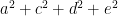. MZ cotwins in their turn share all genetic and environmental influences on their phenotypes other than the non-shared environmental variance, so the MZ covariance equals total variance minus the unshared environment: . On the other hand, under random mating, DZ cotwins share an expected 50 percent of their additive genetic variants, all of their shared environment, and 25 percent of their non-additive genetic variants, leading to the DZ covariance expression .[Note 1] That the weight of the shared environment is the same in MZ and DZ twins reflects the equal environments assumption.

Following the approach in Jöreskog (2021a), the ACDE model can be written as a system of three equations:

is the phenotypic variance across all twins, is the MZ covariance, and is the DZ covariance. While these three are unobserved population parameters in the formal sense, they can always be readily estimated from data, and thus are never unknown in the equations presented in this post. The unknowns are the four variance components , , , and .

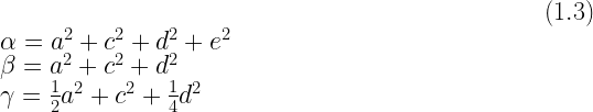
The first equation in (1.3) can be simplified with the help of the second equation:

As and are known, the estimate for can now be readily calculated by rearranging the equation: . With classical twin data, can always be estimated. However, there are still three unknowns in the second and third equations of (1.3), which is the basic problem with the ACDE model. There are infinitely many values of , , and that provide an exact solution to the equations. Sets of feasible values can be generated by substituting some value for one of the unknowns, and then solving for the other two.

The most popular way to deal with the ACDE underidentification problem is to set the value of to zero, which is equivalent to assuming that all genetic effects on the phenotype are additive. This gives us the ACE model:

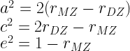
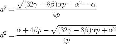
Now there are three equations and three unknowns, so a unique solution is available. Through basic algebraic manipulations, we can express the three unknown parameters in terms of the known variance and covariances:

Substituting a sample variance and sample covariances for , , and will give estimates for , , and .

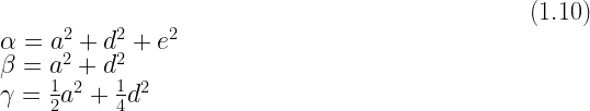
Jöreskog develops his model in matrix form, so it is useful to do the same here. The ACE model can be written as the following matrix equation which is equivalent to (1.3) after the removal of the terms:

The coefficient matrix is square and full rank, so a good way to solve for the unknowns is to multiply both sides with the inverse of the coefficient matrix, which gives the same ACE solutions as in (1.6):

So far, we have retained the original units of the phenotype, but if we want to calculate standardized effect sizes (or proportions of variance), we must take ratios of the unstandardized estimates. For example, heritability is:

, the broad heritability, equals , but because the ACE model presupposes that , the narrow heritability is the same as . For example, if , , and (the hat symbol indicates that we are dealing with sample estimates rather than population values), the unstandardized ACE estimates are:

And therefore the heritability estimate is:

In the interests of generality, in this post I focus on twin models that produce unstandardized parameter estimates.[Note 2] However, standardized estimates can always be calculated as ratios of the unstandardized estimates, as above. In some examples I will use variance decompositions where the total variance equals 1, in which case the unstandardized and standardized models are the same model.

The ACE model fits most datasets fine, but if the MZ covariance is more than twice the DZ covariance, the ACE model estimate will be negative. Considering that is a variance component, this does not generally make sense. Instead, the MZ covariance being more than twice the DZ covariance suggests there are non-additive genetic effects. Accordingly, the value of in (1.3) can be set to zero, leading to the ADE model:

This is equivalent to the following matrix equation:

This coefficient matrix is invertible as well, so the equation can be solved by multiplying both sides with the inverse of the matrix:

At first blush, these estimators may seem mystifying. Why is it that, say, twice the MZ covariance minus four times the DZ covariance is expected to equal , the non-additive genetic variance? The answer is that given the assumption that phenotypic differences are caused by uncorrelated causes, the desired quantity, such as , can be obtained by finding a linear combination of MZ and DZ (co)variances which has a correct amount of the desired cause and none of the other causes. For example, the MZ and DZ covariances under the ADE model are equal to and , respectively. It is a matter of simple arithmetic that two of the former minus four of the latter will leave just one standing.

2. Jöreskog’s ACDE model

While the ACE and ADE models provide estimates of behavioral genetic parameters, they are based on the untested assumption that a particular parameter value is zero. This is a suboptimal approach with an obvious risk of bias, so Jöreskog’s claim that it is possible to estimate the full model without such uncertain assumptions is intriguing.

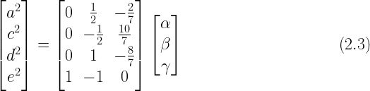
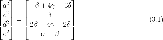
Jöreskog’s ACDE model can be represented by this matrix equation which is equivalent to the system of equations presented in (1.3) above:

There are four unknowns (, , , and ) but only three equations, so the matrix is not invertible, and there are an infinite number of solutions. All vectors that are consistent with the following constraints provide an exact solution to the underdetermined system:

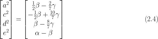
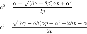
A unique value can be calculated for . This is not possible for , , and . Some additional constraint must be introduced if unique estimates for all parameters are to be obtained. Jöreskog proposes to do this by using the Moore-Penrose pseudoinverse, which exists for all matrices, including ones that are not square and that have deficient rank. When a rectangular matrix has linearly independent rows, as in this case, the right pseudoinverse can be used. If the underdetermined system of equations is , the Moore-Penrose solution is . When this is applied to (2.1), we get:

In this system, there is a one-to-one relationship between the unknown parameters and the known values , , and .[Note 3] A unique set of parameter estimates is therefore available:

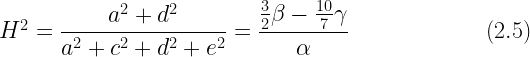
Standardized parameter estimates can be computed as ratios of the unstandardized estimates. For example, broad heritability is equal to:

However, on the face of it, this solution is absurd. Why would this particular set of parameter estimates be anywhere close to the truth? For example, why would the additive genetic variance be equal to half the MZ covariance minus two sevenths of the DZ covariance? Quantitative genetic theory suggests no such thing.

To illustrate the problem, let’s say we have a phenotype with a variance of 1, and MZ and DZ covariances of 0.70 and 0.40, respectively (when the variance is 1, covariances are equivalent to correlations). The following variance decompositions are all consistent with the solution set given in (2.2):

Model	$a^2$	$c^2$	$ d^2$	$e^2$	$ var$	$cov_{MZ}$	$ cov_{DZ}$	$H^2$
$ \text{I}$	$ 0.60 $	$ 0.10$	$ 0.00$	$ 0.30$	$ 1.00$	$ 0.70$	$ 0.40$	$ 0.60$
$ \text{II}$	$ 0.45$	$ 0.15$	$ 0.10$	$ 0.30$	$ 1.00$	$ 0.70$	$ 0.40$	$ 0.55$
$ \text{III}$	$ 0.375$	$ 0.175$	$ 0.15$	$ 0.30$	$ 1.00$	$ 0.70$	$ 0.40$	$ 0.525$
$ \text{IV}$	$ 0.15$	$ 0.25$	$ 0.30$	$ 0.30$	$ 1.00$	$ 0.70$	$ 0.40$	$ 0.45$
$ \text{V}$	$ 0.075$	$ 0.275$	$ 0.35$	$ 0.30$	$ 1.00$	$ 0.70$	$ 0.40$	$ 0.425$
$ \text{Joreskog}$	$ 0.24 $	$ 0.22$	$ 0.24$	$ 0.30$	$ 1.00$	$ 0.70$	$ 0.40$	$ 0.48$

Innumerable different combinations of , , , and will give rise to the same MZ and DZ variance-covariance matrices. While estimates from Jöreskog’s model, presented in the last row of the table, satisfy equation (2.2), too, why would this particular solution be the optimal one? Unfortunately, Jöreskog does not discuss this crucial issue. He simply presents the Moore-Penrose solution as the solution to the ACDE model. But how does this algorithm arrive at a unique set of parameter values?

The answer is simple. When the Moore-Penrose inverse is used to solve an underdetermined system with more unknowns than equations, it selects from among the infinite feasible solutions the one that minimizes the Euclidean norm, which is also known as the norm. The Euclidean norm is the distance of a vector from the origin, and it is calculated as the square root of the sum of the squares of the vector’s entries. In the present case, this means simply that the solution that Jöreskog’s model provides is the one that minimizes the sum of the squares of the entries of the parameter estimate vector (the square root can be ignored because for non-negative and ). Because the model parameters are squared quantities (, etc.), this means that the quantity to be minimized is the sum of the fourth powers of , , , and :

The solution is the vector whose squared entries have the smallest sum among all the vectors that satisfy equation (2.2). It is easy to see what kind of vectors fulfill this criterion best. Firstly, because squared quantities increase faster than linearly, it is better to have more rather than fewer non-zero entries in the vector whose distance from zero is being minimized. For example, it is better to have two parameters that each account for 40 units of variance than a single parameter that accounts for 80 units. This is because is more than . Secondly, it is better to spread the variance evenly rather than unevenly among the parameters because, for example, .

Therefore, of the infinitely many solutions that perfectly fit the underdetermined system of equations, Jöreskog's model selects the one that spreads the phenotypic variance as evenly as possible among all four parameters. The ideal ACDE solution under this criterion would be for each parameter to get one fourth of the variance, but because the solution must also be consistent with equation (2.2), the ideal can usually only be approximated. Jöreskog gives no theoretical reason for why there would be this tendency towards an even split between these four sources of variance, and it is difficult to come up with one. There may be applications where the Euclidean norm leads to a reasonable approximation in the absence of other information, but behavioral genetics is not one of those applications.

The biases of Jöreskog’s estimators are easy to investigate by plugging the model-implied values of the twin variance and covariances from (1.3) into the formulas in (2.4). The asymptotic expected values, , of Jöreskog’s estimates are:

Only the estimator is unbiased. The asymptotic expected values of the , , and estimates are arbitrary-seeming linear combinations that are essentially unrelated to the true values of the parameters. Jöreskog’s estimators will therefore never produce estimates that approximate the true values, except by chance.

To confirm that Jöreskog’s estimates reflect only the minimization described in (2.6), in the Appendix I show that his ACDE estimators can be derived using constrained optimization. Furthermore, a popular method for minimizing the norm is ridge regression, which suggests that the ridge estimator could be used to obtain Jöreskog’s estimates. This is indeed the case, as I also show in the Appendix.

3. Euclidean norm versus parsimony

Many mathematical criteria other than the Euclidean norm could be used to come up with a solution to the underidentified ACDE model, leading to quite different sets of parameter estimates. For example, one could argue that parsimony should be favored, and in that case the ACE model which explains the data in the table in the previous section with three parameters (Model I) would obviously be preferred to the full ACDE model that requires four parameters to account for the same data. It could even be said that Jöreskog’s model reflects the principle of anti-parsimony, or Occam’s butterknife, with the most convoluted answer regarded as the best one. For example, even if the MZ covariance is exactly twice the DZ covariance, and the data are therefore consistent with the two-parameter AE model, Jöreskog’s approach will produce an ACDE solution where the variance is distributed approximately equally between the four parameters. Considering that many lines of evidence point to the AE model being the mechanism behind the typical complex human trait (Hill et al., 2008; Polderman et al., 2015), a widespread adoption of Jöreskog’s ACDE model would lead to a severely skewed understanding of genetic and environmental determinants of human variation.

An ACDE estimator that favors parsimony can be implemented with linear programming. The “norm” equals the number of non-zero entries of a vector, so when it is minimized, the result is parsimonious. In the Appendix, I present an R program that minimizes . For example, if the phenotypic variance is 1, the MZ covariance is 0.70, and the DZ covariance 0.40, the program gives the following solutions:

	$ a^2$	$ c^2$	$ d^2$	$ e^2$
$ L^0$ solution 1	0.60	0.10	0.00	0.30
$ L^0$ solution 2	0.00	0.30	0.40	0.30

The first solution is the ACE model, which at three parameters is more parsimonious than the ACDE model, but there is also a second, equally parsimonious solution, the CDE model. While the CDE model is algebraically feasible, it is very improbable–interactions without main effects are unusual in general, and non-additive genetic variance in the absence of additive genetic variance may well be impossible for a polygenic trait in any population that is not highly inbred.

Let’s assume that , , , and , resulting in a variance of 1 and MZ and DZ covariances of 0.85 and 0.40, respectively. minimization gives two optimal solutions given these twin data:

	$ a^2$	$ c^2$	$ d^2$	$ e^2$
$ L^0$ solution 1	0.75	0.00	0.10	0.15
$ L^0$ solution 2	0.00	0.25	0.60	0.15
Joreskog	0.31	0.15	0.39	0.15

The ADE and CDE models are now the parsimonious solutions. However, both are biased as the true model is ACDE. Jöreskog’s ACDE decomposition of these covariances, shown in the last row, is closer to the mark, but still quite biased. Even when ACDE is the true model, Jöreskog’s estimates will be satisfactory only by chance.

As should be obvious from these examples, there is no reason to believe that the Euclidean norm, parsimony, or any other mathematically convenient criterion would produce ACDE estimates that are anywhere close to the true population values. If the full model is to be estimated, there are no substitutes for acquiring additional data that are informative about , , or . For example, if we knew the phenotypic covariance between genetically unrelated individuals raised together, call it , it would be simple to expand the model in equation (2.1) so that the full ACDE model could be estimated. The estimates would then be:

4. Discussion

Jöreskog (2021a) proposed to estimate the ACDE model by using the Moore-Penrose inverse. This enabled him to come up with estimates for all four parameters (, , , and ) while using only classical twin data. However, this “trick” makes sense only if the minimization of the Euclidean norm–essentially the sum of the squares of the parameters–is a good way of getting at the genetic and environmental determinants of phenotypic differences. Jöreskog puts forward no argument that this would be the case, and I do not think any reasonable argument of the sort can be made. In other words, there are no realistic circumstances in which Jöreskog’s estimators can be expected to produce anywhere close to unbiased estimates, and typically the estimates will be grossly biased. The model is simply a non-starter, and it should not be used for any purpose. Nor can any other purely mathematical criterion help make the ACDE model identified in a useful way, which means that ACE, ADE, and the other identified but possibly biased submodels of ACDE are usually the only practical options.

ACE is the most commonly used twin model. It assumes that genetic effects are purely additive, but if this is not the case, estimates will be biased. Nevertheless, I would argue that the bias is not too serious in typical settings. The asymptotically expected amount of bias can be found by plugging an ACDE decomposition in the and estimators given in (1.6):

When non-additive genetic effects are present, the ACE estimate of genetic variance in (4.1) does not approximate the additive genetic variance, but is instead an inflated estimate of the total genetic variance (or the unstandardized broad heritability). The expected inflation factor is equal to , and the shared environmental variance is simultaneously underestimated by the same amount, as seen in (4.2). However, both theory and data suggest that is typically very small in magnitude for complex human traits, so the bias in ACE estimates is likely to be slight (Hill et al., 2008; Mäki-Tanila & Hill, 2014; Hill & Mäki-Tanila, 2015; Polderman et al., 2015; Hivert et al., 2021a, 2021b; see also [Note 1]). A violation of the assumption that will therefore typically not lead to markedly erroneous inferences about the relative importance of genes versus the environment. The relative importance of additive versus non-additive heredity may be somewhat more strongly misestimated, though. In any case, the biases of the ACE model under non-additive heredity are negligible compared to those of Jöreskog’s model under any circumstances, cf. (2.7) above.

Another thing to consider is that human mating is not random with respect to many socially valued phenotypes studied by behavioral geneticists. This means that bias in ACE estimates due to a neglect of non-additive heredity is often counterbalanced by an opposite bias due to the unmodeled effects of assortative mating. Moving from random mating to (positive) assortative mating increases phenotypic variance in the same way in MZ and DZ twins.[Note 4] It does not change the MZ genetic correlation (which is always perfect), but it increases the DZ additive genetic covariance in relation to the MZ additive genetic covariance, so that the former will now be more than half the size of the latter, on average. If p is the phenotypic correlation between parents and mate selection is based directly on phenotypic similarity, the expected covariance of DZ twin offspring under the ACDE model is (see Lynch & Walsh, 1998, p. 158):

where is narrow heritability, and is, as usual, unstandardized, so that and are generally not equal. A further assumption in that equation and in those that follow is that assortative mating has been going on at the same level of intensity for several generations, reaching an equilibrium where the surplus variance it creates does not change between generations — in (4.3) as well as in (4.4) and (4.5) is the equilibrium variance, and is narrow heritability at equilibrium. The effect of assortative mating on non-additive variance is negligible for highly polygenic traits, and it is assumed to be zero here. If ACE estimators are used in the presence of both non-additive genetic variance and assortative mating, the parameters are asymptotically expected to be biased in the following way (as usual, the estimate is not affected):

The genetic variance estimate in (4.4) approximates the total genetic variance and is still affected by the upwardly biasing term, but there is now also a downwardly biasing term which equals . Similarly, the estimate in (4.5) is deflated by but also inflated by . This means that there is often an automatic stabilization or regularization effect inherent in the ACE model whereby biasing but opposite influences tend to offset each other. The resulting parameter estimates are more robust to model violations than the apparent simplicity of the model would suggest. For example, if , , , , and , the ACE estimates are[Note 5]:

While ACE is not the model that generated the data, the heritability estimate nevertheless equals broad heritability, and the shared environment estimate is right on the mark. In real data, the result would probably not be as perfect, but the fact that biases in the ACE model frequently go in opposite directions does tend to blunt the distortionary effects of model violations. This kind of mutual canceling may also explain why the DZ covariance is often not more than half the MZ covariance for phenotypes that are known to be subject to positive assortative mating.

Contrary to the notion that progress is genomics would swiftly make twin studies and kinship-based behavioral genetics in general obsolete, twin and family studies remain essential for understanding human genetics. While these traditional methods cannot estimate the genetic values of individuals, they nevertheless have certain advantages over genomic methods.

A particular problem with genomic methods is population stratification which means that the apparent effect of genetic locus G on phenotype P may not be causal () but can instead reflect a correlation between G and environmental factor E which is the true cause (). If this is not controlled for, genomic estimates will be biased. Twin and family methods by their very nature control for stratification by varying genetic relatedness while holding the environment constant, or vice versa. This is why methodological criticisms of twin research have focused on what could be called within-family stratification, such as the supposedly different environments that MZ and DZ twin pairs experience (on this point, see my post on the equal environments assumption). The fact that family methods control for stratification is why perhaps the leading method of validating findings from genome-wide association studies is replicating them in family samples (e.g., regressing sibling phenotypic differences on sibling polygenic score differences).

Another advantage of twin and family methods is that they can estimate the total genetic variance, while genomic methods have so far tended to be limited to the effects of genetic variants that are common (e.g., with a population frequency greater than 1 percent). Whole-genome data and genomic methods for analyzing related individuals make the bridging of this gap possible, and the expectation is that genomic estimates of heritability will converge to those from twin and family studies. Until either all of family-based heritability for a given trait has been explained genomically, or any discrepancies between family and genomic estimates have been convincingly resolved otherwise, there is no full explanation of familial phenotypic resemblance. Triangulation with different methods subject to different weaknesses is a traditional approach to debiasing estimates in behavioral genetics, and it comes to good use when genomic and kinship-based estimates are harmonized.

Notes

1. Non-additive genetic effects are referred to with the symbol D or d, but it should be noted that in the classical twin design this source of influence includes both dominance and epistasis, not just dominance. This is so because the MZ correlation for all genetic effects, additive and non-additive, is 1, while the DZ correlation is for both dominance and epistasis. In other words, an interaction between two alleles within a locus (dominance) and between two loci (epistasis) increases twin similarity in the same way, making dominance and epistasis one and the same phenomenon from the perspective of twin modeling.

This symmetry breaks down if there is higher-order epistasis which means that three or more alleles interact with each other. The MZ correlation is 1 for all higher-order effects, too, while the DZ correlation for each effect is , which means that the DZ correlation decreases as n, the number of interacting loci, increases. This means that the more complex and influential the allelic interactions are, the more similar MZ twins will be compared to DZ twins. Theoretically, there could be a trait whose variance were entirely due to high-order interactions, so that the MZ correlation would be 1 while the DZ correlation would be ~0.

However, both empirical and theoretical evidence indicates that non-additive genetic variance is unlikely to pose serious problems to twin modeling. Firstly, if non-additive variance and higher-order interactions in particular were major determinants of phenotypic variance, MZ twin pairs would commonly be much more than twice as similar as DZ twins. In their meta-analysis of almost 18,000 traits in 14.5 million twin pairs, Polderman et al. (2015) found that for 69 percent of traits, the observed twin correlations were consistent with a model where twin resemblance was solely due to additive genetic variation, i.e., MZ twins were twice as similar as DZ twins. For most of the traits for which this model was inadequate the MZ pairs were less than twice as similar as DZ pairs, which is also inconsistent with non-additive genetic variance being a major determinant of phenotypic differences. Thus only a small proportion of traits show evidence of important gene interactions, contradicting the notion that complex interactions, rather than genetic and environmental main effects, are essential to explaining human differences.

Non-additive genetic variance has also been investigated with genomic methods. These methods fail to support the idea that dominance or epistasis would be important causes of phenotypic differences in humans (Pazokitoroudi et al., 2021; Hivert et al., 2021a). Consistently with the twin data, genomic methods suggest that the non-additive genetic contribution could be zero for the typical trait. In the behavioral domain, Okbay et al. (2022) notably found no evidence for dominance effects on educational attainment in a well-powered genome-wide association sample of 2.5 million people. (The existence of recessive mental retardation syndromes and inbreeding depression indicate that dominance effects on educational attainment are non-zero, but such effects cannot be observed in GWASs. Given the rarity of these conditions, at least in developed countries, the proportion of population variance that they contribute must be very small.)

Several theoretical and mathematical explanations of the observation that genetic variance is overwhelmingly additive have been developed. The basic insight of these arguments is that even if there is non-additive gene action in individuals, it does not necessarily translate into non-additive genetic differences between individuals. Rather, much or all of the non-additive influence will be reflected in the additive (or average) effects of loci. Hill et al. (2008) argued that the allele frequency distributions of human traits are usually U-shaped, with most frequencies close to 0 or 1, causing the average effects to account for essentially all of the variance even when there is dominant or epistatic gene action.

Mäki-Tanila & Hill (2014) emphasize that all “the epistatic terms involving a particular locus appear in its average effect”, which means that epistasis as such does not lead to large epistatic variance. They report that both uniform and U-shaped allele frequency distributions result in mostly additive variance, while frequencies close to 50 percent yield the most epistatic variance, although with a large number of loci epistatic variance will be low for all frequencies. For example, the frequency distribution of the nearly 4,000 genome-wide significant effect alleles in the educational attainment GWAS by Okbay et al. (2022) is roughly uniform (and would be more U-shaped if rare alleles were observed):

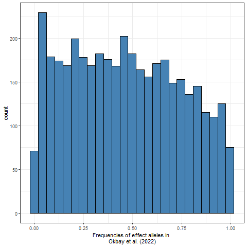
A predominance of allele frequencies close to 50 percent would be expected only in artificial selection experiments, which also helps explain why high epistatic variances have been reported in some studies on model organisms. Mäki-Tanila & Hill (2014) also point out that “epistatic variance is almost entirely contributed by the two-locus epistatic variance”, indicating that higher-order interactions are not expected to contribute much. This suggests that the assumption in twin modeling that the DZ correlation for non-additive genetic effects is always is not too unrealistic.

These considerations indicate that non-additive genetic variance will not be a large source of phenotypic variance for many, or any, complex human traits. Nevertheless, it may often be a small source of variance, and its omission from twin models may cause some bias.

Unmodeled gene-environment interaction is another potential source of bias. It is similar to non-additive genetic variance in that it is often postulated to be important but in practice can rarely be observed with any reliability. It also seems that similar mathematical arguments that point to the rarity of dominance and epistatic variance could be made regarding gene-environment interaction variance.

2. If unstandardized effects are of no interest, the ACE model can also be estimated by using MZ and DZ correlations. The fact that there are multiple estimates of phenotypic variance is ignored, which means that the resulting estimates concern only proportions of variance, not the absolute amounts of variance explained by each parameter. The MZ and DZ phenotypic variances are therefore allowed, in principle, to differ by any amount, whereas unstandardized ACE models must either constrain MZ and DZ variances to equality, or to explicitly include unequal variances in the model specification. The standardized ACE model is:

The estimators are:

and are intraclass correlations.

3. Jöreskog describes (1.6), (1.12), and (2.4) as maximum likelihood estimators, but as far as I can see, maximum likelihood is incidental to this approach, used only to estimate , and , and some ancillary statistics, rather than the actual parameters of interest. Instead, the essence of the method is the matching of the moments of (joint) distributions to functions of the model parameters, which is the hallmark of the method of moments. Maximum likelihood is the most popular method for estimating twin models, but it typically involves the iterative maximization of a likelihood function so as to minimize the differences between the model-implied twin matrices and the observed twin matrices. Jöreskog’s estimates may satisfy the ML criterion, but he does not demonstrate it.

4. Under random mating the effects of genetic loci are uncorrelated (assuming that other mechanisms, e.g., natural selection, do not cause correlations), so that the total variance of the effects of all loci equals the sum of the variances of the effects. In contrast, under assortative mating the total variance equals the sum of the variances of the effects plus their covariances. This comes from a basic relationship between variances and covariances:

The covariances between effects for each locus are zero under random mating, while under positive assortative mating the covariances are positive, leading to increased variance. If there is disassortative mating (“opposites attract”), the covariance terms will be negative, and the genetic variance will be smaller than under random mating. However, it seems dubious whether disassortative mating exists in humans, other than in the trivial case of the perfect negative correlation between the parents’ sexes.

If (positive) assortative mating stays at the same level for several generations, additive genetic variance will reach a constant equilibrium value that is higher than the additive genetic variance under random mating. If p is the parental phenotypic correlation and is narrow heritability under assortative mating, $ a^2$ and $ \tilde{a}^2$ are related in the following way (Lynch & Walsh, 1998, p. 158):

This formula can be used to estimate how much lower the additive genetic variance of the trait would be without assortative mating.

5. Method-of-moments ACE and ADE estimators that accommodate assortative mating can be derived from (1.6), (1.12), and (4.3).

The ACE estimators are:

The ADE estimators are:

The assumption in both sets of estimators is that assortative mating has been going on for several generations while p, the parental phenotypic correlation has remained constant, and therefore has reached an equilibrium level. Another assumption is, of course, that or is zero, and if that is not case, the resulting estimates may be more biased than those based on the ordinary ACE and ADE estimators–this is because of the mutually canceling biases of the latter. The estimates are unstandardized, and standardized quantities like heritability can be calculated as ratios of each estimate to the total variance in the usual manner. Estimates of are not affected by assortative mating.

References

Hill, W. G., Goddard, M. E., & Visscher, P. M. (2008). Data and theory point to mainly additive genetic variance for complex traits. PLoS Genet., 4, e1000008.

Hill, W. G., & Mäki-Tanila, A. (2015). Expected influence of linkage disequilibrium on genetic variance caused by dominance and epistasis on quantitative traits. J. Anim. Breed. Genet., 132, 176–186.

Hivert, V., et al. (2021a). Estimation of non-additive genetic variance in human complex traits from a large sample of unrelated individuals. Am. J. Hum. Genet., 108, 786–798.

Hivert V., Wray N. R., & Visscher, P. M. (2021b). Gene action, genetic variation, and GWAS: A user-friendly web tool. PLoS Genet 17(5): e1009548.

Jöreskog, K. G. (2021a). Classical models for twin data. Structural Equation Modeling: A Multidisciplinary Journal, 28, 121–126.

Jöreskog, K. G. (2021b). Classical Models for Twin Data: The Case of Categorical Data. Structural Equation Modeling: A Multidisciplinary Journal, 28, 859–862.

Lynch, M., & Walsh, B. (1998). Genetics and Analysis of Quantitative Traits. Sunderland, MA: Sinauer Associates.

Mäki-Tanila, A., & Hill, W. G. (2014). Influence of gene interaction on complex trait variation with multilocus models. Genetics, 198, 355–367.

Neale, M.C., & Maes, H.H.M. (2004). Methodology for genetic studies of twins and families. Dordrecht, NL: Kluwer Academic Publishers.

Okbay, A., et al. (2022). Polygenic prediction of educational attainment within and between families from genome-wide association analyses in 3 million individuals. Nature Genetics, 54, 437–449.

Pazokitoroudi, A., et al. (2021). Quantifying the contribution of dominance deviation effects to complex trait variation in biobank-scale data. Am. J. Hum. Genet., 108, 799–808.

Polderman, T. J. C., et al. (2015). Meta-analysis of the heritability of human traits based on fifty years of twin studies. Nature Genetics, 47, 702–709.

Appendix

Lagrange multipliers

Jöreskog’s model can also be estimated with the method of Lagrange multipliers. This method allows for the minimization of an objective function that is subject to equality constraints.

With $ a^2, c^2, d^2$, and $ e^2$ denoted by $ A, C, D$, and $ E$ for convenience, the objective function to be minimized is:

$ f = A^2 + C^2 + D^2 + E^2$

Equation (2.2) provides three constraints (the fourth is the identity $ d^2 = d^2$ which is of no use here) that are arranged so that all non-zero terms are on the same side:

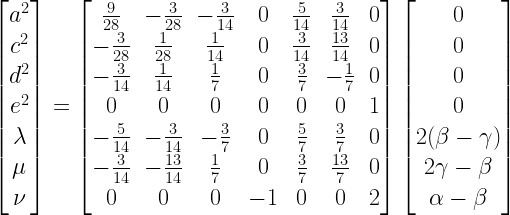
The Lagrangian function is:

where the three Greek letters are the unknown Lagrange multipliers.

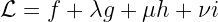
The partial derivatives of $ \mathcal{L}$ with respect to $ A, C, D$, and $ E$ are:

The four partial derivatives, when equated to 0, and the three constraints form a system of seven linearly independent equations in seven unknowns:

This system can be solved by multiplying both sides with the inverse of the coefficient matrix:

The solution is:

These values of $ a^2, c^2, d^2$, and $ e^2$ match exactly with the pseudoinverse solution presented in equation (2.4), and given that $ f$ is a strictly convex function, the values are where $ f$ reaches its minimum. This confirms that Jöreskog’s estimates are equivalent to

which, alas, provides no basis for estimating behavioral genetic parameters.

Ridge regression

Ridge regression minimizes the $ L^2$ norm, and can be used for underdetermined systems, so it should be equivalent to Jöreskog’s method. The estimator is:

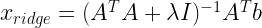
Applying it to equation (2.1), we get:

This results in a rather complex expression:

However, is the shrinkage parameter, and we are not interested in shrinking the estimates towards zero, so itself can be set to zero. This greatly simplifies the solution:

As expected, the answer matches the pseudoinverse solution in equation (2.4).

Ridge regression is typically used to mitigate the effects of multicollinearity in regression models with many highly correlated independent variables. It reduces the variance of the estimates in exchange for some bias. However, while ridge regression can be used to solve the underdetermined ACDE model, it is not a reasonable use case for it. The results are so biased that they are worthless.

Sparse solutions to the ACDE model

The $ L^0$ “norm” denotes the number of non-zero entries of a vector. Minimizing the $ L^0$ “norm” results in a parsimonious, or sparse, solution where there are as many zero entries as feasible. A sparse solution to the ACDE model is one where the parameter estimate vector $ \begin{bmatrix} a^2 & c^2 & d^2 & e^2 \end{bmatrix}^T$ contains as many zero entries as possible given the constraints stated in equation (2.2).

The $ L^0$ minimization problem can be solved iteratively with mixed integer linear programming. $ a^2, c^2, d^2$, and $ e^2$ are denoted $ A, C, D$, and $ E$ for convenience and to emphasize that for the optimizer they are just numbers, rather than squares of anything (polynomials involved in linear programming can be at most degree 1). The objective function to be minimized is the number of non-zero entries in $ \{ A, C, D, E \}$. The constraints describing the set of all feasible solutions are given by equation (2.2), with phenotypic variance and MZ and DZ covariances fixed to some observed values.

In the program, there is a binary count variable accompanying each continuous variable A, C, D, and E, and additional constraints are set up so that each binary variable gets a value of 0 when its associated continuous variable is zero and a value of 1 when the associated continuous variable is non-zero (this is a variant of the Big M method). The optimizer then finds solutions to the constraints that minimize the sum of the binary count variables. I used the R package lpSolve to do the optimization:

#install.packages("lpSolve")
#install.packages("lpSolveAPI")
library(lpSolve)
library(lpSolveAPI)

# twin variance and covariances
varMZDZ <- 225
covMZ <- 125
covDZ <- 38

# auxiliary constant to prevent small (co)variances from messing up the counting constraints
if(varMZDZ < 3) 
aux <- 0.99 else 
aux <- 0

# set the number of variables
model <- make.lp(0, 8)

# define the objective function; the 1s signify equal weights
set.objfn(model, c(0, 0, 0, 0, 1, 1, 1, 1))

# counter variables are binary
set.type(model, c(5, 6, 7, 8), "binary")

# set constraints to define the feasible solution set
add.constraint(model, c(1, 0, 1.5, 0, 0, 0, 0, 0), "=", 2*(covMZ - covDZ))
add.constraint(model, c(0, 1, -0.5, 0, 0, 0, 0, 0), "=", 2*covDZ - covMZ)
add.constraint(model, c(0, 0, 0, 1, 0, 0, 0, 0), "=", varMZDZ - covMZ)

# set constraints to count nonzero parameters
add.constraint(model, c(-1, 0, 0, 0, 1, 0, 0, 0), "<=", aux)
add.constraint(model, c(1, 0, 0, 0, -1*(covMZ), 0, 0, 0), "<=", 0)
add.constraint(model, c(0, -1, 0, 0, 0, 1, 0, 0), "<=", aux)
add.constraint(model, c(0, 1, 0, 0, 0, -1*(covMZ), 0, 0), "<=", 0)
add.constraint(model, c(0, 0, -1, 0, 0, 0, 1, 0), "<=", aux)
add.constraint(model, c(0, 0, 1, 0, 0, 0, -1*(covMZ), 0), "<=", 0)

# set the upper and lower bounds
set.bounds(model, lower=c(0, 0, 0, 0, 0, 0, 0, 0), upper=c(covMZ, covMZ, covMZ, varMZDZ - covMZ, 1, 1, 1, 1))

# compute the optimized model
solve(model)
solution_number <- 1

# get the minimized value of the objective function
objective <- get.objective(model)

# lpSolve does not automatically report multiple solutions at the same level of sparsity, so the program will loop until all maximally 
# sparse solutions have been found, with a new constraint equivalent to the previous solution added after each loop
while (objective == get.objective(model) & objective<10) {
cat("\n\nOptimal solution #", solution_number)
cat("\nNonzero parameters:", get.objective(model))
cat("\na^2: ", get.variables(model)[1])
cat("\nc^2: ", get.variables(model)[2])
cat("\nd^2: ", get.variables(model)[3])
cat("\ne^2: ", get.variables(model)[4])
add.constraint(model, c(0, 0, 0, 0, get.variables(model)[5:7], 0), "<=", sum(get.variables(model)[5:7])-1)
solve(model)
solution_number <- solution_number + 1
}

At least one of $ \{ A, C, D \}$ can always be set to zero while satisfying the constraints–that is the logic behind the practice of fixing D or C to zero when estimating ACE and ADE models. The optimizer will therefore always find at least one solution that is more sparse than the full ACDE model.