In his recent book Hive Mind economist Garett Jones argues that the direct effect of IQ on personal income is modest, and that most of the benefits of higher IQ flow from various spillover effects that make societies more productive, boosting everyone’s income. This, he says, explains the “IQ paradox” whereby IQ differences appear to explain a lot more of the economic differences between nations than within them.
Jones does not say in his book what he thinks the exact effect of IQ on personal income is, but on Twitter he has asserted that “Fans of g would do well to look at the labor lit: 1 IQ point predicts just 0.5% to 1.2% higher wages.” He has also said that, in terms of standardized effect sizes, IQ accounts for only about 10% of variance in personal income (a correlation of ~0.32).
While I don’t doubt Jones’s overall thesis that the effect of IQ on productivity is broader than its effect on personal productivity or income, I think he understates the importance of IQ in explaining income differences between individuals. I analyzed a large American population sample and found a substantially larger effect of IQ on permanent income than previous investigations. It appears that the literature Jones refers to has failed to pay sufficient attention to various measurement issues.
Measuring Permanent Income
There are two biasing influences that make measures of income available in many datasets highly inadequate. First, due to transitory fluctuations in income and reporting errors, an individual’s reported income may differ considerably from one year to another, which means that a single-year income may present a misleading picture of his or her income in a typical year. Secondly, there’s a lifecycle bias in income whereby income measured when an individual is too young or too old may be a poor guide to his or her long-term consumption and investment possibilities, given that income trajectories over time may differ between individuals.
Permanent income is the idea that income consists of a permanent component and a transitory component, and that it is the permanent component that we want to know if we wish to study the determinants of differences in financial success. Mazumder (2015) argues that to get a good estimate of permanent income one must calculate an average income centered on age 40 when the lifecycle bias is minimized. Ideally, one would average annual income reports from perhaps age 25 to age 55, that is, starting when most people have finished their education and stopping before many people have retired. (To give an example of how much the adequate measurement of income matters: Mazumder found that the intergenerational elasticity of income is around 0.6-0.7 in America when parental income is measured by averaging parents’ incomes over several decades. This compares to estimates of around 0.3-0.4 found when parental income is measured based on one or at most a few years.)
Some studies cited by Jones use measures of average hourly wage and the like, but annual income seems to me to be a more intuitive choice, especially if we are comparing the effects of IQ on GDP and personal income. So, I’ll concentrate on permanent annual income in this post.
Data
I used data from the NLSY79 which is an ongoing longitudinal study that follows the lives of a large sample of Americans born in 1957-64. Specifically, I used the nationally representative subsample comprising more than 6000 individuals.
The NLSY79 contains income data collected from individuals annually until 1994 and every two years thereafter. Using these data, I calculated a measure of permanent income for each individual, following Mazumder’s recommendations to the extent that the data allowed it.
My permament income measure is the average income calculated from up to nine biennial income reports from age 32 or 33 to age 47 or 48. The following table shows which years were used for each cohort:
| Birth year | Income years used |
|---|---|
| 1957, 1958 | 1989, 1991, 1993, 1994, 1997, 1999, 2001, 2003, 2005 |
| 1959, 1960 | 1991, 1993, 1995, 1997, 1999, 2001, 2003, 2005, 2007 |
| 1961, 1962 | 1993, 1995, 1997, 1999, 2001, 2003, 2005, 2007, 2009 |
| 1963, 1964 | 1995, 1997, 1999, 2001, 2003, 2005, 2007, 2009, 2011 |
2011 is the most recent year with data, and all earlier income figures were converted to 2011 dollars using the Consumer Price Index.
There are reports of income from a number of different sources in the NLSY79. Only two of these — salaries, wages, and tips and net business and farm income — were used in the calculation of my permanent income measure; the rest, such as unemployment compensation and capital gains, were excluded. Both of the variables used are top-coded so that all values above a cutoff — which was \$100,000 in 1989-1993 and the top 2% ever since — have been replaced with the average of the values above the cut-off. If a respondent didn’t have reported income from either source for at least five of nine possible years, he or she was excluded from the analysis. Respondents reporting a permanent income of zero were also dropped. This led to a sample size of 4615.
The permanent income is, therefore, the average annual income from employment and self-employment between the ages 32/33 and 47/48. Permanent income did not differ significantly between cohorts (secular stagnation?), so I did not residualize the variable for birth year. The following graph shows how permanent income is distributed in the NLSY79 sample:

The natural logarithm of the same variable looks like this:

For IQ scores, I used the AFQT percentile scores that had been renormed for age in 2006 by the NLS staff. The test was administered when most of the participants were in their late teens to early 20s. Using the van der Waerden formula, I converted the percentile scores to normal scores that have a mean of 100 and a standard deviation of 15. These normal scores were used in all the analyses that follow.
The following tables shows IQ statistics for the full nationally representative NLSY79 sample and selected subgroups:

5.6% of the sample was excluded for not having valid IQ scores, as shown in the first table.
More exclusions resulted from the fact that not everybody had reported data allowing the calculation of their permanent income. The following table shows summary statistics for the permanent income sample drawn from the full sample, along with statistics for selected subgroups:

The size of the permanent income sample is 4451, compared to N=6111 in the full sample. Therefore, 24% of the sample was excluded due to missing data, largely reflecting the fact that many working-age people are in fact not working on a regular basis. The mean IQ is slightly higher and the IQ variance slightly lower in the permanent income sample compared to the full sample.
Results: Overall Picture
I started by regressing my permanent income measure on IQ for all available individuals. The sample should be reasonably representative of American men and women who were born around 1960 and are regularly employed. I used both the untransformed variable (income in dollars) and the natural logarithm of income in dollars.
Here’s the scatterplot and the parameter estimates for the untransformed variable:

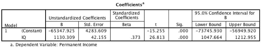
When the dependent variable is income in dollars (not logged), the unstandardized slope coefficient is 1130 (95% CI: 1048-1213), which is the amount of dollars associated with a 1 IQ point change. The expected permanent annual income difference between people who differ by 15 points in IQ is 15*1123=16,950 dollars. The standardized coefficient, or correlation, is 0.37 and the R squared is 14%.
This analysis should be interpreted with caution given the strong non-linearities in the data. In subsequent analyses, I concentrate on log-transformed income which suffers less from this problem.
Here’s what the scatterplot and the parameter estimates look like when the natural logarithm of permanent income is regressed on IQ:

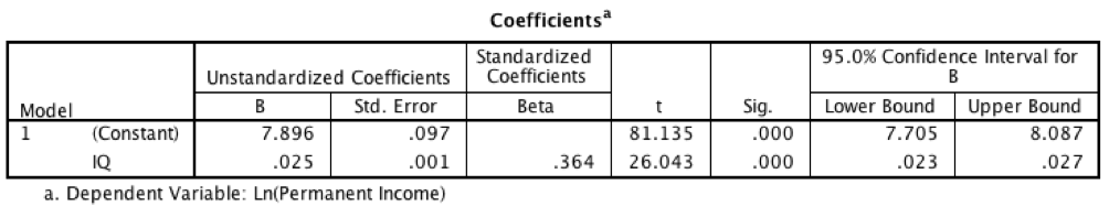
The unstandardized slope coefficient is 0.025 (95% CI: 0.023-0.027). Because the dependent variable is logarithmic, this coefficient, when multiplied by 100, can be (approximately) interpreted as the percent change in income in (unlogged) dollars associated with a 1 IQ point change.[Note] Therefore, one additional IQ point predicts a 2.5% boost in income. The standardized effect size, or correlation, is 0.36 and the R squared is 13%.
These estimates are clearly larger than those reported by Jones. He gave an upper bound of 1.2% for the marginal effect of one IQ point, but I find that the effect is more than twice that. This means that a standard deviation increase in IQ predicts a rise of e^(15*2.5%)-1≈45% in income. For example, the expected permanent annual income for those with IQs of 85 is \$22,490, while it is 45% more, or \$32,730, for those with IQs of 100, and 45% more than that, \$47,620, when IQ is 115, and so on.
Results: By Subgroups
Various subgroup affiliations have been found to moderate the relationship between IQ and income. In particular, the relationship is not necessarily the same for both sexes and for all races and ethnicities.
Let’s look at sex first. I regressed log income on IQ, a sex dummy (men=0, women=1) and a sex dummy * IQ interaction term. The results are below.

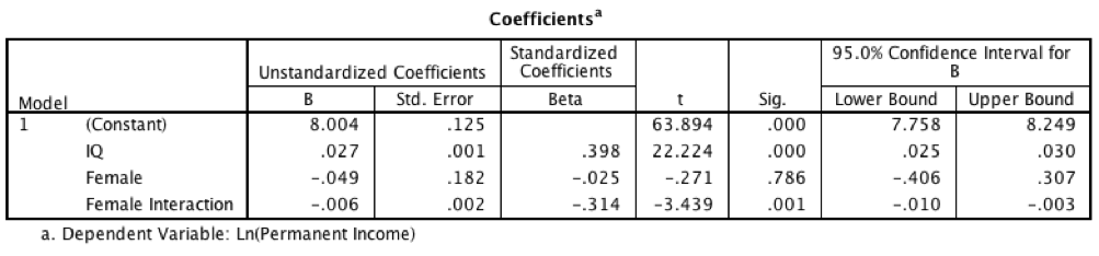
The male slope coefficient is 2.7% (95% CI: 2.4%-3.0%) while the female one is significantly lower, 2.1% (95% CI: 1.8%-2.4%). Each extra IQ point brings 0.6 percentage points more income to men compared to women. The female intercept is smaller, too, but not significantly. Therefore, the following equations can be used to predict the incomes of males and females:
Incomemale = e^(8.004 + 0.027 * IQ)
Incomefemale = e^(8.004 + 0.021 * IQ)
For example, the expected permanent annual income of a man with an IQ of 100 is e^(8.004 + 0.027 * 100), or \$44,530. The expected permanent annual income of a woman with the same IQ is e^(8.004 + 0.021 * 100), or \$24,440.[Note]
When analyzed separately, the R squared is 23% for men but only 9% for women, corresponding to correlations between IQ and income of 0.48 and 0.30 for men and women, respectively. The scatterplot suggests that the lower variance explained by IQ in women is mainly due to the existence of a substantial number of women with little income at all IQ levels. The most important explanation for this is probably that many women are not the primary breadwinners in their families, and are therefore less likely to realize their full income potential.
Given the clearly different regression equations for men and women, subsequent analyses were done separately for men and women.
To analyze the effect of race/ethnicity on the relation of IQ and income, I created dummy variables for blacks and Hispanics, with whites as the reference group, and IQ * race interaction terms for blacks and Hispanics. (The “white” group comprises everybody who is not black or Hispanic, but for these cohorts this group is almost completely white.) The results for men are shown below. It should be noted that the parameter estimates are much more precise for whites than non-whites due to differences in sample sizes.


The slope coefficient for white men (the reference group) is 2.5% (95% CI: 2.2%-2.7%). The Hispanic parameter estimates are not significantly different from the white ones, so the same equation applies to white and Hispanic men, although given the low sample size for Hispanics, this cannot be asserted very firmly. Black men, in contrast, have a significantly lower intercept and a significantly higher slope coefficient: each additional IQ point predicts 3.6% (95% CI: 2.6%-4.5%) more income for black men. The R squared for the entire model is 23%. When analyzed separately, IQ explains 20% of income differences in whites, 18% in blacks, and 16% in Hispanics. The correlations are 0.45 (white), 0.42 (black), and 0.39 (Hispanic). The following equations can be used to predict the permanent incomes of white/Hispanic and black men:
Incomewhite/Hispanic men = e^(8.285 + 0.025 * IQ)
Incomeblack men = e^(7.122 + 0.036 * IQ)
The expected annual income of a white or Hispanic man with an IQ of 100 is e^(8.285 + 0.025 * 100), or \$48,290. A black man with the same IQ can expect an income of e^(7.122 + 0.036 * 100) ~ \$45,340. For those with IQs of 115, the predicted permanent income is \$70,260 for whites/Hispanics and \$77,810 for blacks. These are, as always, expected incomes, that is, mean incomes for that IQ level, with much individual variation around that mean.
Low-IQ black men earning less than low-IQ non-black men even when the marginal benefit of IQ is greater for blacks is something that has been observed before (Nyborg & Jensen, 2001). This finding may be largely due to the fact that a disproportionate share of low-IQ black men are involved in crime and poorly attached to the labor market.
Next, I looked at women of different races/ethnicities using the same model as above. The results are below.


For white women (the reference group), the slope coefficient of IQ on permanent annual income is 2.1% (95% CI: 1.8%-2.5%). Black and Hispanic parameter estimates are larger but not significantly so. In separate regressions, the R squared for whites is only 8%, compared to 14% for Hispanics and 15% for blacks. This difference probably reflects the fact that white women are more often able to rely on their husbands for financial support, and the gap between their potential and actual incomes, given their IQs, is therefore larger than for non-white women.
IQ and Income at Selected Ages
To test how much averaging annual income figures to get a measure of permanent income influences the IQ slope, compared to if income was measured based on single-year reports, I regressed log income at selected ages on IQ using the same sample (not disaggregated by sex or race/ethnicity). The results are shown in the table below.
| Approximate age | Unstandardized slope | Correlation |
|---|---|---|
| 25 | 0.015 | 0.22 |
| 33 | 0.021 | 0.31 | 40 | 0.022 | 0.31 |
| 47 | 0.022 | 0.30 |
The sample size is >3000 for each age, so the estimates are precise. The unstandardized slope is 0.015 at age 25 and about 0.022 at older ages. The correlation is 0.22 at age 25 and about 0.31 thereafter. For comparison, the same parameter estimates were 0.025 and 0.36, respectively, when the permanent income measure was used.
If the transitory component in income was just random noise, you would expect the unstandardized coefficient to be the same for single-year income and permanent income, while the standardized coefficient (correlation) would be somewhat lower for single-year income. However, both estimates appear to be somewhat lower for single-year income.
It’s notable that in the NLSY79, the slope coefficient is higher (0.015) than the upper bound (0.012) suggested by Jones even at age 25 when the effect of the lifecycle bias is strong.
National IQ and GDP
The main argument in Jones’s book is that a nation’s average IQ is much more important for national prosperity than an individual’s IQ is for his or her personal prosperity. Specifically, he has argued that the effect on income is 6-12 times larger for nations than for individuals.
I regressed the natural logarithm of PPP-corrected GDP per capita on national IQ, with data from here (filename Megadataset_v2.0j.csv, variables LV2012measuredIQ and GDPpercapitaPPPcurrentinternational). The scatterplot and the parameter estimates are below.
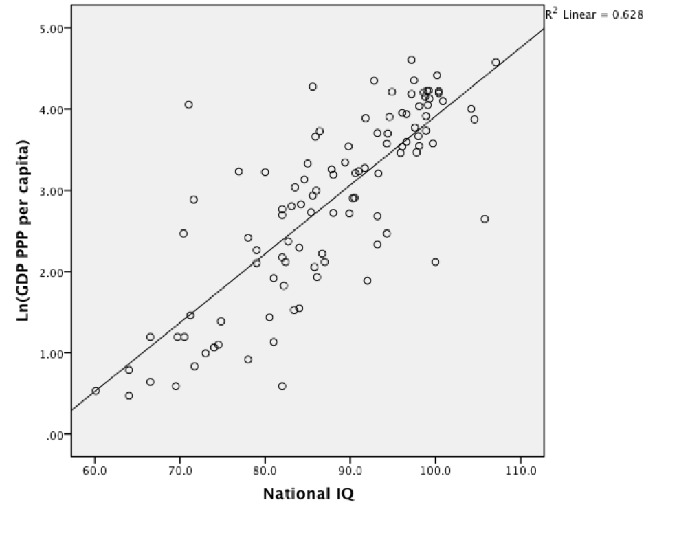

The slope coefficient is 0.085 (95% CI: 0.072-0.097), indicating that a 1 point increase in national IQ predicts an 8.9% increase in GDP per capita. This estimate is about 3.6 times larger than the estimate for the effect of individual IQ in the NLSY79. Jones’s suggestion that the international effect is 6-12 times larger than the individual one appears to be an exaggeration. (The correlation and thus the R squared are much larger in the international IQ regression, but this reflects the fact that it’s an ecological correlation between group averages, with within-group variance suppressed.)
Discussion
I found that in the NLSY79, a large longitudinal dataset with excellent income data, the effect of IQ on personal income, in terms of the unstandardized slope coefficient (which indicates the expected, or mean, amount of income conditional on a given IQ score, without regard to variability around that mean), was about 100-400% larger than what Garett Jones has suggested. Subgroup analyses indicated that this result is very robust across demographic groups.
In terms of variance explained, I found that IQ typically explains more than 10% (which is the effect size Jones has suggested) although this is not true for all demographic groups — the R squared is relatively low in white women, in particular. Jensen (1998) suggested that the correlation of IQ and income in mid-career is 0.40, and this seems like a reasonable overall estimate for the IQ-permanent income correlation, too; the effect is probably somewhat larger than 0.40 for males and somewhat less than 0.40 for females.
It is not clear why my estimates are larger than earlier ones. I would argue that the measure of income I use is superior to those used in other studies. Some of the difference is undoubtedly due to a failure to consider the lifecycle bias in some studies. Other studies may have measures of income that are systematically biased in some other way, and some IQ measures used may be of poor quality, too.
I also tested if my higher estimates were due to the inclusion of both employment and self-employment income, but the parameter estimates were highly similar even when the permanent income measure was based on just one of these income sources. Nor is the larger-than-previously-suggested effect size confined to the NLSY79. I ran some preliminary analyses on the NLSY97 sample, and found that the slope coefficient was substantially higher than 0.012 in this dataset, too.
My analysis suggests that while the “IQ paradox”, as defined by Jones, definitely exists, it appears to be smaller than he has claimed. When GDP per capita is regressed on national IQ, the regression coefficient may be only 3.6 times or so larger than the corresponding coefficient from the regression of permanent income on IQ. Given that some of the apparent effect of national IQ is probably due to reverse causality, the true gap between these two coefficients may be even smaller.
Limitations in my analysis include the fact that I didn’t try to control for people’s participation in the labor market. There are some variables in the dataset that would allow this. I could also have used broader measures of income. Additionally, I didn’t try to account for measurement error in IQ, which means that all of my estimates are somewhat downwardly biased. My permanent income variable is based on five to nine annual income reports, making it much more reliable than the variables used in previous research, but it nevertheless falls short of a perfect measure of permanent income in terms of coverage of the entire working life.
References
Jensen, A.R. (1998). The g factor: The science of mental ability. Westport, CT: Praeger.
Jones, G. (2015). Hive Mind: How Your Nation’s IQ Matters So Much More Than Your Own. Stanford, CA: Stanford Economics and Finance.
Mazumder, B. (2015). Estimating the Intergenerational Elasticity and Rank Association in the US: Overcoming the Current Limitations of Tax Data. Working Paper.
Nyborg, H., & Jensen, A.R. (2001). Occupation and income related to psychometric g. Intelligence, 29, 45-55.
Appendix
Here’s my SPSS code for creating the permanent income variable and certain other variables. First, it calculates the average of employment and self-employment income for each year and adjusts for inflation. Then it calculates permanent income for each cohort. Finally, it calculates incomes for selected ages.
COMPUTE  INCOME_1982=SUM(R1024001, R1024301) * 2.33097.
COMPUTE  INCOME_1983=SUM(R1410701, R1411001) * 2.25842.
COMPUTE  INCOME_1984=SUM(R1778501, R1778801) * 2.16496.
COMPUTE  INCOME_1985=SUM(R2141601, R2141901) * 2.09051.
COMPUTE  INCOME_1986=SUM(R2350301, R2350601) * 2.05236.
COMPUTE  INCOME_1987=SUM(R2722501, R2722801) * 1.98010.
COMPUTE  INCOME_1988=SUM(R2971401, R2971701) * 1.90143.
COMPUTE  INCOME_1989=SUM(R3279401, R3279701) * 1.81402.
COMPUTE  INCOME_1990=SUM(R3559001, R3559301) * 1.72103.
COMPUTE  INCOME_1991=SUM(R3897101, R3897401) * 1.65153.
COMPUTE  INCOME_1992=SUM(R4295101, R4295501) * 1.60327.
COMPUTE  INCOME_1993=SUM(R4982801, R4983201) * 1.55667.
COMPUTE  INCOME_1995=SUM(R5626201, R5626601) * 1.47598.
COMPUTE  INCOME_1997=SUM(R6364601, R6365001) * 1.40149.
COMPUTE  INCOME_1999=SUM(R6909701, R6911101) * 1.35017.
COMPUTE  INCOME_2001=SUM(R7607800, R7609000) * 1.27012.
COMPUTE  INCOME_2003=SUM(R8316300, R8318200) * 1.22276.
COMPUTE  INCOME_2005=SUM(T0912400, T0913900) * 1.15176.
COMPUTE  INCOME_2007=SUM(T2076700, T2078800) * 1.08487.
COMPUTE  INCOME_2009=SUM(T3045300, T3047500) * 1.04849.
COMPUTE  INCOME_2011=SUM(T3977400, T3979400).
EXECUTE.

DO IF R0000500=57.
COMPUTE PERMANENT_INCOME=MEAN.5(INCOME_1989,    INCOME_1991, INCOME_1993, INCOME_1995, INCOME_1997, INCOME_1999, INCOME_2001, INCOME_2003, INCOME_2005).
ELSE IF R0000500=58.
COMPUTE PERMANENT_INCOME=MEAN.5(INCOME_1989, INCOME_1991, INCOME_1993, INCOME_1995, INCOME_1997, INCOME_1999, INCOME_2001, INCOME_2003, INCOME_2005).
ELSE IF R0000500=59.
COMPUTE PERMANENT_INCOME=MEAN.5(INCOME_1991, INCOME_1993, INCOME_1995, INCOME_1997, INCOME_1999, INCOME_2001, INCOME_2003, INCOME_2005, INCOME_2007).
ELSE IF R0000500=60.
COMPUTE PERMANENT_INCOME=MEAN.5(INCOME_1991, INCOME_1993, INCOME_1995, INCOME_1997, INCOME_1999, INCOME_2001, INCOME_2003, INCOME_2005, INCOME_2007).
ELSE IF R0000500=61.
COMPUTE PERMANENT_INCOME=MEAN.5(INCOME_1993, INCOME_1995, INCOME_1997, INCOME_1999, INCOME_2001, INCOME_2003, INCOME_2005, INCOME_2007, INCOME_2009).
ELSE IF R0000500=62.
COMPUTE PERMANENT_INCOME=MEAN.5(INCOME_1993, INCOME_1995, INCOME_1997, INCOME_1999, INCOME_2001, INCOME_2003, INCOME_2005, INCOME_2007, INCOME_2009).
ELSE IF R0000500=63.
COMPUTE PERMANENT_INCOME=MEAN.5(INCOME_1995, INCOME_1997, INCOME_1999, INCOME_2001, INCOME_2003, INCOME_2005, INCOME_2007, INCOME_2009, INCOME_2011).
ELSE IF R0000500=64.
COMPUTE PERMANENT_INCOME=MEAN.5(INCOME_1995, INCOME_1997, INCOME_1999, INCOME_2001, INCOME_2003, INCOME_2005, INCOME_2007, INCOME_2009, INCOME_2011).
END IF.

DO IF R0000500=57.
COMPUTE INCOME_AGE_25=INCOME_1982.
ELSE IF R0000500=58.
COMPUTE INCOME_AGE_25=INCOME_1983.
ELSE IF R0000500=59.
COMPUTE INCOME_AGE_25=INCOME_1984.
ELSE IF R0000500=60.
COMPUTE INCOME_AGE_25=INCOME_1985.
ELSE IF R0000500=61.
COMPUTE INCOME_AGE_25=INCOME_1986.
ELSE IF R0000500=62.
COMPUTE INCOME_AGE_25=INCOME_1987.
ELSE IF R0000500=63.
COMPUTE INCOME_AGE_25=INCOME_1988.
ELSE IF R0000500=64.
COMPUTE INCOME_AGE_25=INCOME_1989.
END IF.

DO IF R0000500=57.
COMPUTE INCOME_AGE_33=INCOME_1990.
ELSE IF R0000500=58.
COMPUTE INCOME_AGE_33=INCOME_1991.
ELSE IF R0000500=59.
COMPUTE INCOME_AGE_33=INCOME_1992.
ELSE IF R0000500=60.
COMPUTE INCOME_AGE_33=INCOME_1993.
ELSE IF R0000500=61.
COMPUTE INCOME_AGE_33=INCOME_1995.
ELSE IF R0000500=62.
COMPUTE INCOME_AGE_33=INCOME_1995.
ELSE IF R0000500=63.
COMPUTE INCOME_AGE_33=INCOME_1997.
ELSE IF R0000500=64.
COMPUTE INCOME_AGE_33=INCOME_1997.
END IF.

DO IF R0000500=57.
COMPUTE INCOME_AGE_40=INCOME_1997.
ELSE IF R0000500=58.
COMPUTE INCOME_AGE_40=INCOME_1997.
ELSE IF R0000500=59.
COMPUTE INCOME_AGE_40=INCOME_1999.
ELSE IF R0000500=60.
COMPUTE INCOME_AGE_40=INCOME_1999.
ELSE IF R0000500=61.
COMPUTE INCOME_AGE_40=INCOME_2001.
ELSE IF R0000500=62.
COMPUTE INCOME_AGE_40=INCOME_2001.
ELSE IF R0000500=63.
COMPUTE INCOME_AGE_40=INCOME_2003.
ELSE IF R0000500=64.
COMPUTE INCOME_AGE_40=INCOME_2003.
END IF.

DO IF R0000500=57.
COMPUTE INCOME_AGE_47=INCOME_2003.
ELSE IF R0000500=58.
COMPUTE INCOME_AGE_47=INCOME_2003.
ELSE IF R0000500=59.
COMPUTE INCOME_AGE_47=INCOME_2005.
ELSE IF R0000500=60.
COMPUTE INCOME_AGE_47=INCOME_2005.
ELSE IF R0000500=61.
COMPUTE INCOME_AGE_47=INCOME_2007.
ELSE IF R0000500=62.
COMPUTE INCOME_AGE_47=INCOME_2007.
ELSE IF R0000500=63.
COMPUTE INCOME_AGE_47=INCOME_2009.
ELSE IF R0000500=64.
COMPUTE INCOME_AGE_47=INCOME_2009.
END IF.
Discover more from Human Varieties
Subscribe to get the latest posts sent to your email.

Excellent work!
This is going on my HBD Fundamentals page.
See also this tweet by Rosalind Arden.
An excellent analysis for which I am most grateful.
Thanks.
is this published somewhere as a journal paper?
No.
This should be a paper. Would be nice to have something to refer and link to that is checked by people in the field. This data stuff is beyond my level of intuitive understanding.